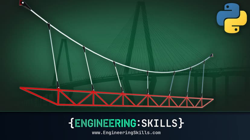
Modelling and Analysis of Non-linear Cablenet Structures using Python and Blender

After completing this course you’ll have developed a complete workflow for the modelling and analysis of non-linear 3D cablenet structures.

We’ll expand beyond what we covered in our study of 2D non-linear cables by adapting the tools we built previously, for the analysis of non-linear 3D cablenet structures.

However, instead of just modifying our existing code, we’ll spend time fleshing out a complete workflow that takes you from initial form-finding of cablenet geometry, right through to iterative stiffness method simulation to identify the cablenet deflections and tension profile.

We can’t embark on the analysis of cablenet structures without making reference to the ‘Godfather’ of cablenet structures, the Architect and Engineer Frei Otto (1925-2015). In fact, we’ll use two of his early tensile structures as the basis for our main case studies.

If you’re intrigued by these elegant and efficient structures and want to understand how to analyse their behaviour, this course is for you. Keep in mind that the tools developed in this course are not meant to be a replacement for commercial non-linear solvers. Our objective is to build your understanding of the behaviour of cablenet structures and geometric non-linearity more generally. The best way to do this is to roll up your sleeves and build your own solver. After taking this course, you’ll be able to use commercial software which a much greater degree of confidence that you understand what’s happening behind the scenes.

While we’re not trying to rebuild SAP2000 or ETABS, when you complete this course you’ll have a range of standalone analysis notebooks. The code developed within each section of the course is also provided for download as a reference.

Course prerequisites

This course picks up where the previous course, Non-linear finite element analysis of 2D catenary & cable structures using Python, left off. You should consider that course a strict prerequisite for this one.

We’ll be using the code developed in that prerequisite course as our starting point in this course. While we’ll recap the key concepts and logic of our iterative solver, we’ll avoid going over old ground in this course. So, even more so than usual, this prerequisite is strongly advised.

If you’ve covered the prerequisite course, you won’t have any trouble with the Python we implement in this course. We’ll develop our Python code using the versatile Jupyter development environment. Unlike the prerequisite course, in this course we’ll use Jupyter Lab. If you’re not familiar with this, don’t worry, we’ll walk through getting Jupyter Lab up and running on your machine.

Course Breakdown

Section 1: Introduction, Course Breakdown & Prerequisites

In this first section, we’ll get our bearings by taking a look at the course structure. This will give you a good idea of what to expect. We’ll also introduce our main focus for this course – cablenet structures. This will provide some context for the technical analysis to follow.

This course assumes that you’ve completed the prerequisite course on 2D cable analysis; we’ll elaborate on why it’s critical that you cover that course first if you want to get the most from this course.

Section 2: Developing the 3D non-linear stiffness matrix

In this section, we’ll take the theory used to develop the 2D non-linear stiffness matrix and extend that to 3D. This really involves two steps; updating how we calculate the element transformation matrix and then updating the local element stiffness matrix. The task here isn’t difficult, the hard work was done in establishing the 2D stiffness matrix in the prerequisite course. We’ll focus on whiteboarding the theory here before diving into code a little later.

Section 3: Extending our Blender Utility Scripts

Blender is a trusty 3D Swiss army knife that makes all of this modelling possible. So, since we’re moving from 2D to 3D, we’ll need to update some of the utility scripts we wrote previously for data import and export. It won’t be all coding in this section, we’ll dabble in some 3D modelling and generate our first simple cablenet model to serve as our test-bed structure for the next section.

Section 4: Extending our solver toolbox from 2D to 3D

Now it’s time to roll up our sleeves and dive into our main solver code. In this section, we’re going to be doing the bulk of the work to update the 2D solver we wrote previously. We’ll also be implementing all of the transformation and stiffness matrix theory we discussed earlier. Once you’ve completed this section you’ll have converted your 2D cable analysis code into a 3D solver…and we can start experimenting with some structures.

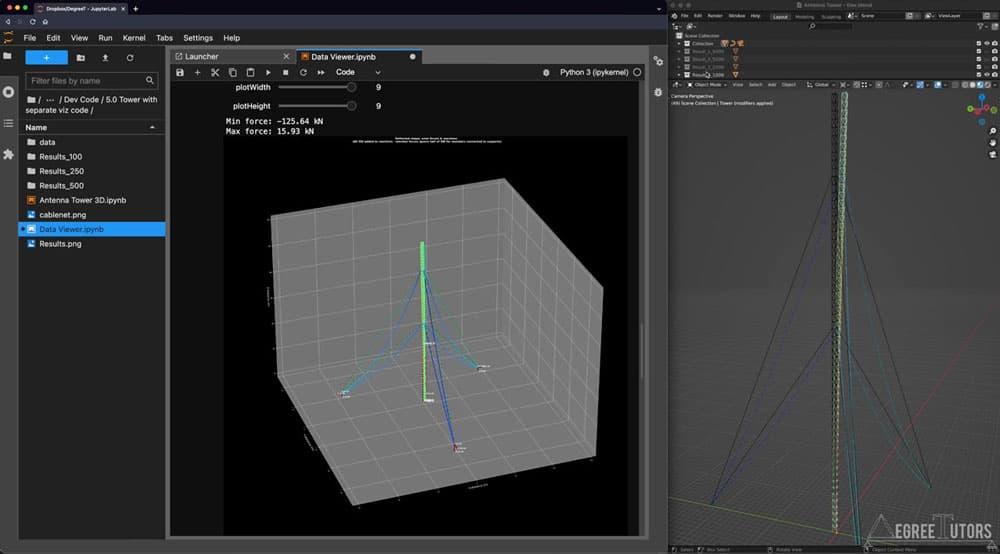
Section 5: Cable-stayed antenna tower…in 3D

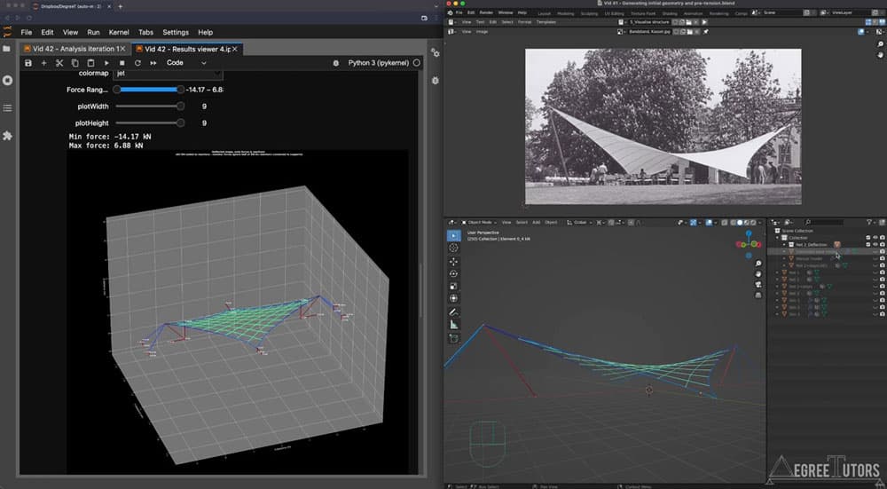
When we studied 2D cable analysis previously, we analysed a 2D cable-stayed antenna tower. So, now that we’ve built ourselves a 3D toolbox, the obvious first task is to build a bigger 3D cable-stayed lattice tower to see how our solver crunches through that! This section will be our first complete run-through of the analysis workflow, from modelling in Blender, to analysis in our solver to results visualisation back over in Blender.

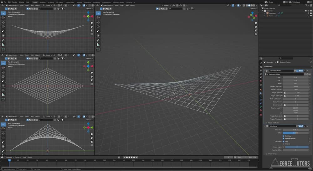
Section 6: Parametric modelling and form-finding in Blender

In this section, we’ll focus on how we can get the most out of Blender’s modelling and simulation tools. We’ll start by exploring Blender’s cloth simulation tools, one of Blender’s many physics engine toolboxes. Although this tool is not designed for structural simulation, it serves as an excellent way of approximating net and membrane geometry which we can use as a starting point for our structural analysis.

We’ll also explore a relatively new feature in Blender; geometry nodes. This functionality gives us the ability to procedurally model and parameterise our geometry. This will be a taster on geometry nodes – after which you can decide if you want to investigate further beyond this course.

This process of exploratory form-finding is one of the most creative and enjoyable parts of studying these structures and serves as a nice counter-balance to our focus on programming and mechanics!

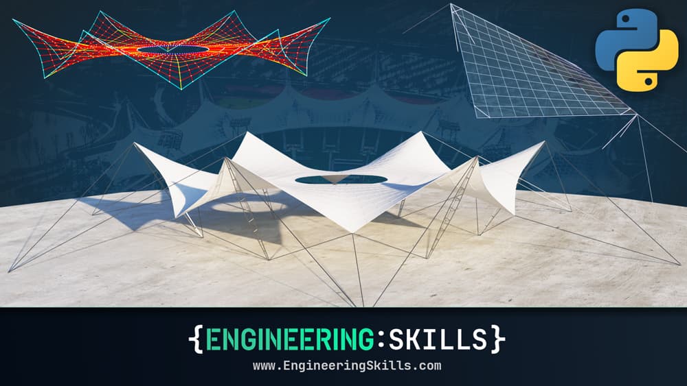
Section 7: Cablenet Pavillion – Hyperbolic Paraboloid

In this section, we’ll bring together our 3D solver with what we’ve learned about form-finding using Blender’s simulation tools. We’ll focus on the modelling and analysis of a hyperbolic paraboloid cablenet structure. For the structure itself, we’ll draw inspiration from a fabric membrane structure by Frei Otto from 1955.

This will give us a good opportunity to discuss the relationship between form-finding and pre-tension. Again, this will be another good demonstration of the typical modelling-analysis-visualisation workflow.

Section 8:Frei Otto’s Dancing Fountain in Cablenet form

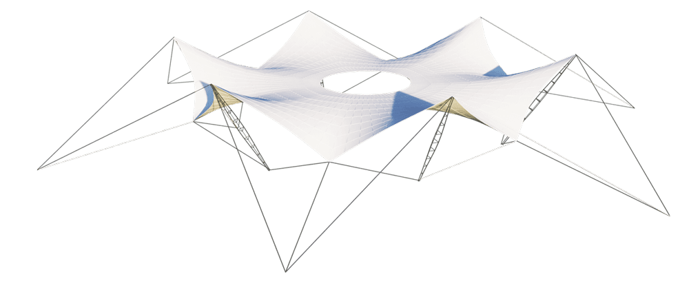
In this final section, we’ll use everything we’ve learned so far to build a model of one of Frei Otto’s finest membrane structures, the so-called ‘Dancing Fountain’ from the Cologne Federal Garden Exhibition in 1957.

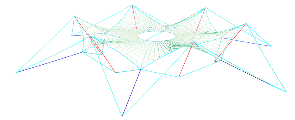
We’ll use all of the tools at our disposal to build the initial geometry, simulate the minimum surface under tension and then analyse the cablenet force distribution under self-weight. Naturally, we’ll bring it all back into Blender for final visualisation.

The successful completion of this structure sets a great high-water mark for your understanding of cablenet structures and of the tools you’ve just built. This should leave you confident enough to explore the behaviour of non-linear cablenet structures in the wild.

Who this course is for

• Students and professional engineers who have completed the 2D non-linear cable analysis course and want to expand into 3D non-linear cablenet structures.
• Students and professional engineers who want to learn more about how to implement iterative methods of analysis in Python.

The codes developed in this course are for educational purposes only and are not tested or certified for use beyond the educational scope of this course. Always employ your own engineering judgement first and foremost, regardless of what the computer says!

Completion certificate

• Download your personalised Certificate of Completion once you’ve finished all course lectures.

• Applying for jobs? Use your Certificate of Completion to show prospective employers what you’ve been doing to improve your capabilities.

• Independently completing an online course is an achievement. Let people know about it by posting your Certificate of Completion on your Linkedin profile or workplace CPD portfolio.

Dr Seán Carroll

BEng (Hons), MSc, PhD, CEng MIEI, FHEA

Hi, I’m Seán, the founder of EngineeringSkills.com (formerly DegreeTutors.com). I hope you found this tutorial helpful. After spending 10 years as a university lecturer in structural engineering, I started this site to help more people understand engineering and get as much enjoyment from studying it as I do. Feel free to get in touch or follow me on any of the social accounts.

---

Do you have some knowledge or expertise you'd like to share with the EngineeringSkills community?

Check out our guest writer programme - we pay for every article we publish.

You Might Also be Interested In...

Non-linear Finite Element Analysis of 2D Catenary & Cable Structures using Python

Build an iterative solution toolbox to analyse structures that exhibit geometric non-linearity due to large deflections.

View Course