A practical guide to floor vibration serviceability assessment
![[object Object]](/_next/image?url=%2Fimages%2Fauthors%2Fsean_carroll.png&w=256&q=75)
Welcome to another EngineeringSkills deep dive. In this two-part tutorial series, we’re going to explore floor vibration serviceability. The core questions that we’re going tackle are;
- how do you quantify the likely vibration response of a floor to occupant-induced footfall forces?
- and how do you determine the acceptability of the predicted response?
By the end of this tutorial, you will have a complete framework for simulating occupant-induced vertical floor vibration and a set of limits against which to compare your predictions. In part two of this series, we’ll build up two working examples in Python that demonstrate the complete calculation workflow.
This series is mainly aimed at working engineers who occasionally find themselves needing to perform design-stage assessments of vibration serviceability. The average civil or structural engineer doesn’t generally work with structural dynamics on a daily basis, - so this guide should act as a helpful primer when the need arises.
It will be helpful to have a working knowledge of structural dynamics fundamentals - if you need a refresher, you can take a look at my course, Fundamentals of Engineering Structural Dynamics with Python.
Fundamentals of Engineering Structural Dynamics with Python
Leverage fundamental structural dynamics to build your own flexible numerical solutions in Python.
After completing this course...
- You’ll understand how to model dynamic behaviour using spring-mass-damper models and how to simulate free vibration behaviour.
- You’ll be able to model the influence of harmonic loading and how to characterise the transient and steady-state responses.
- You’ll be able to use Python to implement the Piecewise Exact Method to model any form of general dynamic loading.
So, with that out of the way, let’s dive in!
1.0 Introduction - the occupant-induced vibration problem
Occupant-induced floor vibration is a serviceability issue, but unlike excessive deflection, it has the potential to be a significant ongoing nuisance to the end user. Thankfully, checking to ensure acceptable vibration performance has become much easier over the last 20 years or so.
As structures have become lighter and, therefore, more susceptible to excitation, the engineering community has responded, dedicating significant research effort to understanding the problem. As a result, numerous design guides have been developed that the working engineer can now turn to.
The guide that we’ll base our discussion on here is, to my mind, probably one of the most straightforward to apply. It’s founded on solid research and a direct application of structural dynamics fundamentals with very limited use of ‘fudge‘ factors to arrive at an outcome.
We’ll be following ‘A Design Guide for Footfall Induced Vibration of Structures’ by Willford and Young and published by the Concrete Centre [1]. Despite the publisher being the Concrete Centre, the guidance is material agnostic.
That said, there is a similar publication aimed at steel structures, ‘Design for Floor Vibrations: A New Approach (P354)‘, published by the Steel Construction Institute (SCI). Both guides follow a broadly similar approach of dividing floors into low and high-frequency structures with low-frequency floors being assessed for resonant response and high-frequency structures being assessed for impulse response.
The SCI guide contains more information on estimating modal properties of steel-specific floorplates. Both are well worth reading, particularly as concise sources of background information on the occupant-induced vibration problem.
Both of the guides cited above are from UK organisations. If you’re in a different part of the world, you’ll likely have local guidance that should be considered. However, the Concrete Centre guidance is so straightforward in its application of fundamental structural dynamics that it should always yield a sensible estimate of response.
It’s worth quickly noting what we’re not covering here; we deal only with vibration in the vertical direction. Lateral or torsional vibrations are far less common in floor structures and, for the most part, are not relevant here.
We’re also not considering the more ’exotic’ case of human-structure interaction, i.e. although the occupants (sources of excitation) may perceive the vibration response, we assume that it has no impact on the dynamic forces they generate.
Human-structure interaction is far more common in the case of lateral vibrations, often seen on footbridge structures. The most notable case of human-structure dynamic interaction was the London Millennium Footbridge. That’s a story for another day…here we’re focusing only on the ‘run of the mill’ nuisance vibration of floors and footbridges.
2.0 Footfall-induced dynamic forces
To assess how humans walking on a floor causes it to vibrate, we need to understand the forces a walking human generates: so-called Ground Reaction Forces (GRF). Volumes have been written in the research community about GRFs. Here, we’ll stick to explaining the bare essentials. Check out the guidance documents cited above for some good background on this.
When we walk, we apply vertical forces (GRFs) to the walking surface as each foot makes contact with it. If we maintain a relatively constant walking speed, these forces are applied at a steady frequency - the walking or pacing frequency.
The time history of successive GRFs represents an approximately periodic force. It’s approximate because GRFs from successive footsteps are not identical - but close enough that approximating the time history as a periodic signal is justified.
So, if we accept that walking pedestrians impose a periodic dynamic force onto the walking surface, we can use Fourier decomposition (as we would on any periodic signal) to represent the force as a summation of sinusoidal force harmonics with varying force amplitude. Each harmonic will have a frequency that is an integer multiple of the fundamental harmonic or pacing frequency (typically between and ).
As an example, let’s say a pedestrian is walking with a swift but fairly typical pacing frequency of and they have a weight . We can represent the force they apply to the walking surface as a combination of their static weight and the dynamic component of the applied force, modelled as a Fourier Series,
where, is the Fourier coefficient (also knows as a Dynamic Load Factor), is the phase of the harmonic.
The last time we discussed this model, we only concerned ourselves with the fundamental harmonic, applied at in our example here. However, for a more robust estimate of floor vibration we need to consider the first four harmonics.
So, this means that our walking pedestrian will apply harmonic forces to the structure at and . Each of these forces will have an amplitude .
The next task is to determine what the is for each harmonic. The most widely cited and applied work on was completed by Kerr [3]. They proposed dynamic load factors for each of the first four harmonics as a function of harmonic frequency. Figure 1 below shows Kerr’s data along with a number of other data sets collected by different researchers.
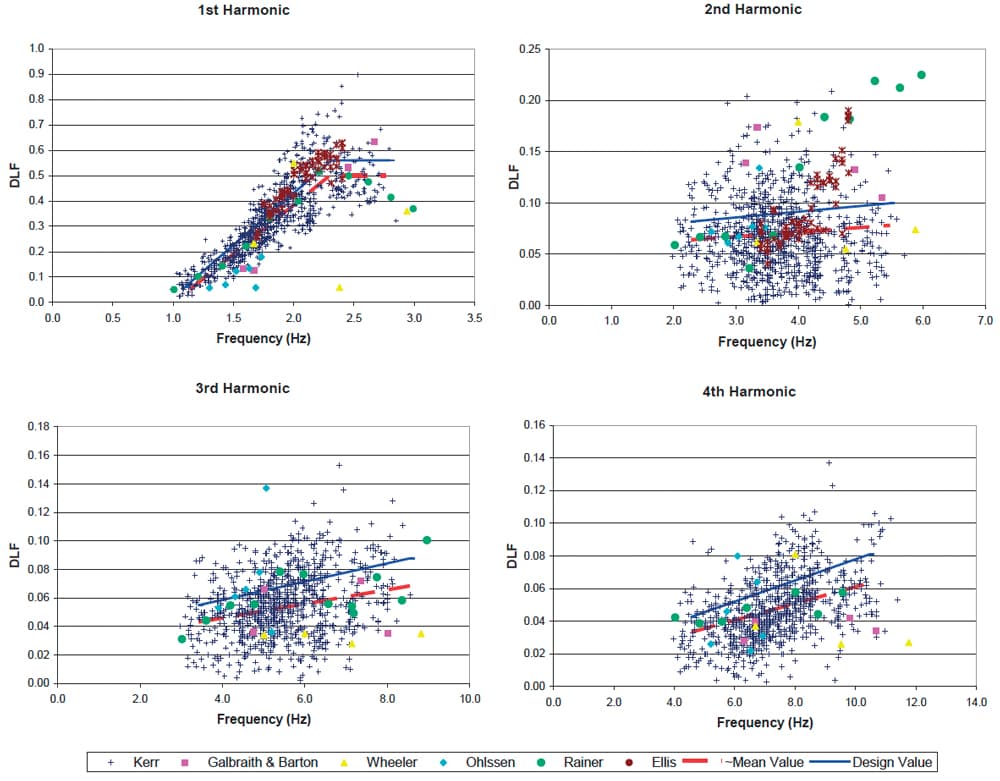
Fig 1. Dynamic load factors for the first four harmonics of the GRF, showing data obtained from Kerr and others [1].
This data has been used to propose empirical expressions for the DLF of each harmonic. These expressions can be used in our analysis and are shown in table 1.
This data has been used to propose empirical expressions for the DLF of each harmonic. These expressions can be used in our analysis and are shown in table 1.
| Harmonic Number | Harmonic frequency, (Hz) | Design DLF |
|---|---|---|
Table 1. Dynamic load factors derived from experimental observations and proposed in [1].
For reference, Table 2 shows the expressions for DLFs proposed in the Steel Construction Institute guidance, [2]. These are slightly more up to date and also reference Kerr’s work as a contributing source.
Both sets of expressions yield very similar DLFs, so similar in fact that an error introduced by using one over the other is insignificant in the face of other sources of error already baked into any design stage analysis. Here, we’ll be using the expressions put forward in [1].
| Harmonic Number | Harmonic frequency, (Hz) | Design DLF |
|---|---|---|
| $7.2-8.8 |
Table 2. Dynamic load factors derived from experimental observations and proposed in [2]. Note that the design DLF is in terms of walking frequency, .
With reference to Fig 1, we can see a strong correlation between increasing walking frequency and for the first harmonic with the correlation becoming less pronounced for higher harmonics.
This data is derived from tests of 882 subjects. The design proposed (Table 1) have a probability of exceedance. The degree to which this dataset captures and accounts for inter-subject variability is a large part of why it is so often cited to this day.
Using these factors and the model in equation 1 above, we can generate a reasonable approximation of the vertical GRF generated by a walking pedestrian.
Although it may not mean much to you now, I’ll say here for completeness, that this model will be applied to floors we designate as low-frequency structures. An alternative model based on modelling the force as an impulse will be applied to high-frequency floors, but we’ll meet that a little later.
3.0 Structural vibration modes and superposition
In the previous section we focused on the applied force - this is one half of the problem. Now, we turn our attention to the other half - the structure. In particular, we need some baseline understanding of how a structure is typically characterised for dynamic analysis.
To analyse a structure’s response to dynamic loading, we could take two routes:
- Build and solve the governing equations of motion directly, or
- Use modal analysis to break the system into a more manageable set of single-degree-of-freedom systems or modes.
Option 2 is by far the more practical and widely adopted approach for civil engineering structures. Again, we’ll focus on the concept of modal analysis at a high level here, but if you want to more deeply understand modal analysis, you can take a look at my course, Multi-Degree of Freedom Dynamics, Modal Analysis and Seismic Response Simulation in Python which goes into the topic in more detail.
Multi-Degree of Freedom Dynamics, Modal Analysis and Seismic Response Simulation in Python
Build the knowledge and tools to decode the dynamic response of real-world structures to real-world loads.
After completing this course...
- You will be able to model the influence of earthquake-induced ground motion.
- You will develop numerical tools to solve the coupled equations of motion for multi-degree of freedom systems.
- You will understand the role of modal decomposition in uncoupling the equations of motion and identifying the underlying dynamic characteristics of MDoF systems.
So, for now, let’s just accept that there is a computational technique we can perform that will yield a set of:
- modal frequencies,
- modal massess,
- and mode shapes,
And that these allow us to model the dynamic response of the structure as the summation of responses from a series of single-degree-of-freedom systems. This is known as model superposition and it’s an incredibly useful technique as it dramatically simplifies the process of dynamic analysis.
For simple structures, we can make use of analytically determined modal properties - that’s what we’ll use in this tutorial. But for production work on real structures, your modal properties will almost certainly be extracted from a finite element model.
Regardless of how the modal properties are determined, the dynamic analysis that follows is the same. We’ll cover the determination of modal properties using finite element analysis of realistic structures in an upcoming tutorial.
Modal analysis is so powerful because it allows us to boil down the dynamic characteristics of the structure into a handful of properties. We can then use these to build a complete picture of how that structure will respond to any dynamic loading.
One thing to appreciate about modal analysis is that it also allows us to immediately identify what forcing frequencies our structure is likely to resonate with. For example, recall our pedestrian walking at above. We know that their GRF has frequency components at and . We can literally interpret this as applying individual sinusoidal forces at each frequency.
So, if our structure has a vertical mode of vibration in the region of say , we know we may have a problem because the harmonic (at ) of the walking force will resonate with the structural mode at . If the walking force is applied for long enough and the structural damping ratio is low enough, the vibration amplitude of the structure may build to a level that is perceived by the occupants and therefore become a problem.
3.1 Damping
The damping ratio is an inherent property of the structure and quantifies its ability to disipate energy. The damping ratio governs the rate at which transient unforced vibration dies out and also influences the maximum response achieved during forced vibration.
Technically, we can determine a damping ratio for each mode, but it is more common to adopt a single damping ratio for all modes, dictated by the type of structure. Damping ratios between and are common for civil structures with values at the lower end used for steel structures and values at the higher end for concrete structures.
The true damping ratio for a structure can only be determined from in-service testing, so estimates are made at design stage based on prior observations. The damping values in the table below are good starting point for design stage calculations.
| Type of structure | Damping ratio, |
|---|---|
| Welded steel bridges with little or no services, fixtures or fittings | |
| Bolted steel, composite and pre-stressed concrete bridges with little or no services, fixtures or fittings | |
| Reinforced concrete bridges | |
| Bare steel composite or post-tensioned concrete floors with little or no fit out | |
| Bare reinforced concrete floors | |
| Completed steel composite or post-tensioned concrete floors with low fit out | |
| Completed steel composite or post-tensioned concrete floors with typical fit out | |
| Completed reinforced concrete floors with typical fit out | |
| Completed steel composite, post-tensioned or reinforced concrete floors with extensive fit out and full height partitions |
Table 3. Suggested damping ratios for various structural forms [1].
4.0 High-frequency versus low-frequency floors
Up to this point, we’ve made several references to so-called low-frequency and high-frequency floors. We classify a floor as being one or the other based on the frequency of its first vertical vibration mode, .
Low-frequency floors are those where the max walking frequency. Otherwise, the floor is classed as a high-frequency floor.
We make this distinction because a low-frequency floor is at much higher risk of resonating with one of the first four harmonics of the GRF. Again, going back to our pedestrian walking at ; their GRF can potentially resonate with any structural mode up to . If we take as the maximum likely walking frequency, we can identify as a practical boundary between low and high-frequency floors.
For a high-frequency floor, resonant response is highly unlikely, however, occupants can still be disturbed by the transient response of the floor to each footfall impact. In this case, we model the GRF from each footstep as an impulse rather than a Fourier series of harmonics.
The procedure for classifying the floor and, therefore, determining the appropriate analysis to perform can be mapped as follows: Fig 2.
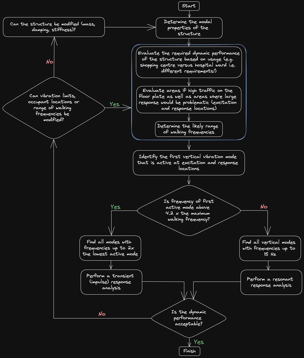
Fig 2. Procedure for floor classification, adapted from [1].
5.0 Human perception and response factors
Human perception of vibration is quite subjective and is influenced by a number of factors. The most relevant to our discussion are the frequency of vibration, the axis of vibration and the duration of exposure. For vertical floor vibration, we’re concerned with human perception to vibration in the z-axis or head-to-toe axis, Fig 3.
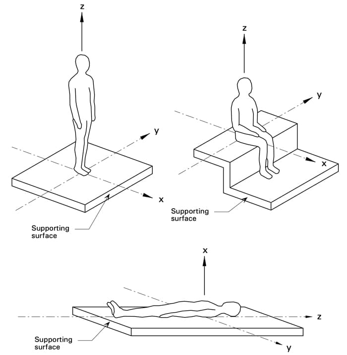
Fig 3. Axes for perception of vibration defined in ISO 2631, BS 6472-1 and BS 6841.
BS 6472 specifies vibration limits that represent the threshold of human perception to continuous vibration as a function of frequency, Fig 4.
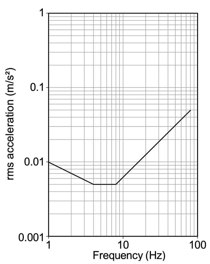
Fig 4. Z-axis base curve for perception of continuous vibration.
The line on this graph is known as an isoperceptability line and represents the boundary or threshold of perception in the z-axis. Note that it is a plot of root-mean-square (RMS) acceleration versus frequency.
The RMS value is a more representative measure of continuous vibration amplitude. We must acknowledge that occupant-induced vibration is unlikely to be continuous. As such, treating it as a continuous vibration source is slightly conservative as tolerance of occupant-induced vibration is likely to be slightly higher due to its intermittent nature.
5.1 Response Factors
A response factor is a multiplier on the base level of perception identified from Fig 4. This is an intuitive and convenient metric we can use to report the vibration performance of a structure. A response factor of 1 corresponds to a vibration response that is only just perceptible, whereas a response factor of 4 is 4 times higher than the barely perceptible level.
We can obtain the response factor by simply dividing the anticipated RMS acceleration (the output from our dynamic analysis) by the baseline acceleration from Fig 4 for the frequency of oscillation. We’ll see this later in example 1 below.
5.2 Limits on continuous vibration
Once we have a response factor, we need to make a judgement on its acceptability. BS 6472 provides guidance on response factors for various environments that should achieve a ’low probability of adverse comment’ from the occupants. These are shown in Table 4 below.
| Environment | Response Factor |
|---|---|
| Critical working areas | 1 |
| Residence (day) | 2-4 |
| Residence (night) | 1.4 |
| Office | 4 |
| Workshop | 8 |
Table 4. Response factors from BS 6472 for ‘low probability of adverse comment’.
Remember, human perception of vibration is subjective, as such the limits in Table 4, should not be treated rigidly, for example, a response factor of 3.9 is not likely to be perceived any differently to a response factor of 4.1. As pointed out in [1], ‘a significant change in perceptibility would generally require a change in vibration level of a factor of 2’. So, observe these limits with a suitable degree of flexibility and don’t make judgements based on a second significant figure!
5.3 Vibration Dose Values
In the event that treating the occupant-induced dynamic loading as continuous is proving too onerous and you need to ‘sharpen the pencil’ to bring home a compliant design, Vibration Dose Value (VDV) assessment offers an alternative to continuous vibration assessment discussed thus far.
The vibration dose value takes into account the intermittent nature of the excitation and effectively allows for a response that would be greater than that allowed for continuous vibration, but only for short periods of time.
If a floor is deemed acceptable under a continuous vibration assessment, there is no need to perform VDV analysis. We won’t consider VDV any further here but you can find good information and examples on its implementation in [2].
6.0 Determining dynamic performance
At this point, we have enough of the background material covered, and we’re ready to start digging into the details of how to actually calculate the structural response.
We’ll start by working through the calculation procedure for low-frequency structures and then cover the procedure for high-frequency structures. Rather than simply stating the equations one after the other as they’re set out in [1], I’ll try to add some additional context and explanation around each equation.
6.1 Low-frequency (resonant) response calculation
For a given walking frequency, , our task is to calculate the magnitude of the steady-state response…
- in each vibration mode of the structure,
- to each of the first 4 harmonics of the ground reaction force.
We can then sum the responses across all modes and calculate a response factor for each mode. Then, we sum the response factors to arrive at a total response factor that maps to the walking frequency, that we started out with.
If we repeat this process for a range of walking frequencies, we can plot the response factors as a function of , giving a complete picture of the likely dynamic behaviour of the structure. The process lends itself quite nicely to a spreadsheet or Python implementation, which we’ll see in part 2. You may find it easier to understand the process set out in a flow diagram, Fig 5.
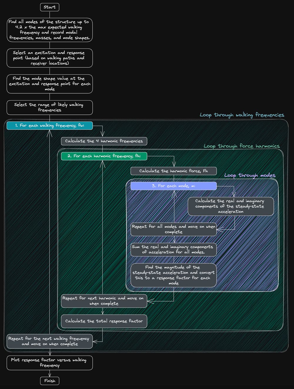
Fig 5. Low-frequency structure resonant response calculation procedure, adapted from [1].
So, for each harmonic of the fundamental walking frequency , we obtain the harmonic forcing frequency, ,
We then obtain the harmonic force, , using the DLFs from table 1,
where is the static weight of the walker. The steady-state acceleration response in each mode is then obtained in terms of its real and imaginary components,
where,
is the modal damping ratio (Table 3), is the modal mass and and are the normalised mode shape values at the selected excitation and response points in the structure.
is a reduction factor than can be applied to account for crossing a span - i.e. it reduces the response to account for the fact that a pedestrian may have crossed the span before the maximum steady-state response has had time to develop. is given by,
where the number of footsteps can be estimated as,
where is the stride length. We can conservatively omit which is more relevant for linear structures like footbridges.
Next, we can sum the real and imaginary components of the response for each mode which gives us the total response for this particular force harmonic,
The total real and imaginary response (all modes superimposed) can then be recombined to obtain the magnitude of the steady-state acceleration response to this force harmonic,
Before continuing with the procedure, let’s pause here to unpick equations (4) through (12) and tie them back to what we know about fundamental structural dynamics.
Recall from Fundamentals of Engineering Structural Dynamics with Python, that the steady-state displacement response of a single-degree-of-freedom (SDoF) system to harmonic excitation is given by:
where:
- is the applied force amplitude ( in Eq. 3),
- is the system stiffness,
- , the frequency ratio ( above),
- is the angular forcing frequency (equivalent to above),
- is the angular natural frequency of the system (equivalent to above),
- is the system damping ratio ( above).
We notice that the response has two components, one in phase with the forcing function,
and one, out of phase with it (indicated by the use of the cosine term),
For clarity, we can temporarily make the following substitution,
Now, dropping the time-varying periodic component, the magnitudes of the components of the steady-state response can be represented as,
and
Although (17) and (18) represents components of displacement amplitude, they are analogous to the components of acceleration amplitude from Eq. 4 and 5 (although 4 and 5 have additional factors , and ).
Since 17 and 18 represent amplitudes of periodic functions, they can be conveniently represented as rotating vectors on the complex plane to better visualise their relation to each other, Fig 6.
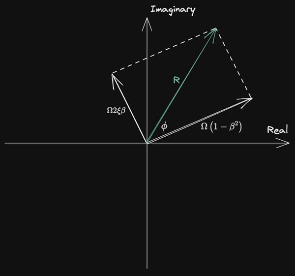
Fig 6. Both components of the steady-state displacement response represented as rotating vectors on the complex plane.
The green vector, which is the vector sum of the two white component vectors, represents the actual steady-state response of the system. Recognising this vector magnitude as the hypothenuse of a right angle triangle with opposite and adjacent sides given by the two component vectors, the steady-state response is given by,
This is what we’re calculating in Eq. 12. Now, reversing the temporary substitution (for ) we just made yields,
Referring back to equations (17) and (18); the component of response given by Eq. 17 is referred to as the real component while the component in Eq. 18 is the imaginary component. This assignment emerges from the alternative complex algebra treatment of the equation of motion. We will give these labels no further attention here - all that is required is that we recognise that both components (real and imaginary) are required to fully capture the complete harmonic oscillation.
So far, we’ve been using a discussion of the basic theory in terms of displacements () to demonstrate the meaning behind equations 4, 5 and 12. Let’s now convert to accelerations and demonstrate direct equivalence between our fundamental theory of dynamics and the equations provided in the guidance document.
Now, from 17 and 18, we see that the magnitude of the real component of the steady-state displacement (the length of the rotating vector) is given by,
and the imaginary component is,
Noting that the steady-state acceleration amplitude is relating to the steady-state displacement by the expression
we can state the amplitude of the real component of the steady-state acceleration as,
and the imaginary component is,
24 and 25 are directly equivalent to 4 and 5 above, except for the application of , and .
We recognise as the reduction factor discussed above. The mode shape factors and take account of the excitation and response location and how these locations influence the estimated response factor for each mode. We’ll see more clearly how these factor into the analysis in our worked examples in part 2.
Now that we understand how the steady-state acceleration amplitude , is obtained for each harmonic of the GRF, we can convert this into a response factor associated with each harmonic, . We do this as discussed above, by dividing by the baseline acceleration (corresponding to a response factor of 1) for each harmonic frequency, ,
can be determined directly from the base curve in Fig 4 or from the equivalent expressions,
Finally, we combine the response factor for each harmonic using the square root sum of the squares for all four GRF harmonics,
Remember, this value of corresponds to a walking frequency of and assumes that the excitation is being applied at a static location, encoded by and that it is being perceived at a static location, encoded by . Assuming the most onerous locations have been chosen for and (these may even be co-located), the analysis should be repeated for all likely walking frequencies.
Alternatively, we may decide to hold the walking frequency constant and repeat the analysis for the full range of excitation and response locations. This allows us to identify where on the structure is most susceptible to excitation for a given frequency. We’ll see examples of both approaches in the worked examples in part 2.
6.2 High-frequency (impulse) response calculation
When evaluating the response of a high frequency structure, we take a slightly different approach. In this case, resonance between any harmonic of the GRF and the structure is unlikely, since the first active mode of the structure is beyond the fourth harmonic of the GRF.
However, occupants can still be disturbed by the vibrations induced by individual footfall strikes. In order to simulate individual forces from each footstep, we apply an ‘effective impulse’ that induces the same peak structural response as the equivalent GRF time-history.
Based on the same experimental work that informed the DLFs from Table 1, the following effective impulse is proposed in [1] for design purposes,
Using this design effective impulse, we can simulate the ground reaction force from successive pedestrian footfalls as a series of impulses applied to the structure.
As this is an impulse, it has units of . It has been empirically shown that the ground reaction force, and therefore the effective impulse, increases with walking speed, therefore it is only necessary to simulate the highest likely walking frequency.
Once the dynamic characteristics of the structure have been determined, the excitation and response locations can be determined (based on the mode shapes).
The analysis procedure is summarised in Fig 7 below.
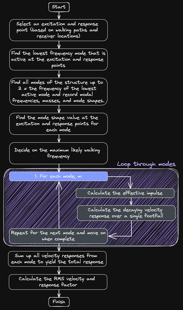
Fig 7. High-frequency structure impulse response calculation procedure, adapted from [1].
We start by performing a modal analysis to identify all modes with frequencies up to twice the fundamental frequency. For each mode, an effective impulse is calculated using Eq. 29.
We then calculate a peak velocity in each mode, ,
We recognise Eq. 30 as being the instantaneous change in velocity induced by the application of an impulse,
where represents the force with magnitude applied for an infinitesimally short duration . In Eq. 30 we interpret the instantaneous change in velocity , as a peak velocity . If you need a refresher on impulse response, we covered this during our discussion of the Duhamel integral in our project on simulating crowd induced vibrations.
Note that the mode shape factors and serve the same purpose here as for low-frequency structures; they encode the position of the excitation and response locations (and the influence their locations have) in the response.
Now that we have the peak velocity induced by an impulse, we can simulate the decaying free vibration response that follows,
The exponential term simulates the decay in response due to structural damping until the next impulse is applied. Note that the duration of this free vibration response , is equal to the period of the pacing frequency,
The total velocity response, is then obtained by summing the individual modal responses,
where is the number of modes considered.
The root-mean-square velocity is then determined,
The we can calculate a response factor by dividing by the baseline velocity, corresponding to a response factor of one.
Note that the response factor here is being evaluated for the fundamental frequency only. Recall back when we evaluated the response factor for low-frequency structures, we evaluated one for each mode and then combined them using the square root sum of the squares.
This is because the low-frequency analysis is a ‘driven oscillation’ problem, i.e. we are driving the structure by applying forces of different (harmonic) frequencies.
However, the high-frequency analysis is a ‘free oscillation’ or ‘free vibration problem’ since we are observing free vibrations of the structure after each impulse is applied. As such, the frequency of oscillation experienced by the occupant, according to this model, will be the fundamental frequency for the structure. This why the response factor is determined for this frequency only.
We can determine the baseline velocity for the fundamental frequency , using the following expression,
Finally, we can express the response factor as,
7.0 Conclusion to Part 1
At this point in our exploration of occupant-induced vibration we’ve covered all of the theory. You should understand:
- how we model occupant-induced dynamic forces,
- the distinction between low and high-frequency structures,
- why we make this distinction and how the analysis procedures for each are implemented,
- the origins of the design equations provided in [1].
However, my guess is that there’s still a lot of uncertainty in your mind about the fine grain detail of implementing the analyses described above. We can only really eliminate that uncertainty by working our way through some design examples - that’s what we’re going to do in 'Part 2: Calculating response factors for floor vibration and assessing performance'. It’s one thing to read about how an analysis is implemented, it’s another thing completely to work through its’s implementation, step-by-step. So, head over to part 2 to see how it’s done.
If you’ve found the structural dynamics content in this tutorial a little challenging, take a look at my Fundamentals of Engineering Structural Dynamics with Python. This is a first introduction to structural dynamics and covers probably about of what you need to know about dynamics as a civil/structural engineer.
Fundamentals of Engineering Structural Dynamics with Python
Leverage fundamental structural dynamics to build your own flexible numerical solutions in Python.
After completing this course...
- You’ll understand how to model dynamic behaviour using spring-mass-damper models and how to simulate free vibration behaviour.
- You’ll be able to model the influence of harmonic loading and how to characterise the transient and steady-state responses.
- You’ll be able to use Python to implement the Piecewise Exact Method to model any form of general dynamic loading.
Ok, that’s it for now - see you over in part 2.
-
[1] ‘A Design Guide for Footfall Induced Vibration of Structures’ by Willford and Young and published by the Concrete Centre
-
[2] ‘Design for Floor Vibrations: A New Approach (P354)‘, published by the Steel Construction Institute
-
[3] Kerr, S.C., Human Induced Loading on Staircases, PhD Thesis, University of London, 1998
Dr Seán Carroll's latest courses.


Featured Tutorials and Guides
If you found this tutorial helpful, you might enjoy some of these other tutorials.
Plastic Analysis and Plastic Collapse – A Complete Guide – Part 1
Use plastic analysis to determine the collapse load factors for determinate and indeterminate structures.

Callum Wilson
Bonsai BIM - The Essential IFC Tool for Structural Engineering Workflows
The IFC tool every structural engineer should have in their toolkit

Petru Conduraru


