Truss Analysis using the Direct Stiffness Method
![[object Object]](/_next/image?url=%2Fimages%2Fauthors%2Fsean_carroll.png&w=256&q=75)
In this tutorial we are going to take a close look at how to use the Direct Stiffness Method to perform truss analysis. By the end of this, you should understand:
- the basic ideas behind why the direct stiffness method works.
- how to execute the analysis technique for truss structures that experience axial forces (2D plane trusses).
- the scalability of the technique and why it’s the main process that powers commercial structural analysis software.
If you want to learn how to implement the direct stiffness method in Python and build your own truss solver (without previous coding experience), consider taking this course where I walk you though the process from setting up Python to running your 2D truss solver.
The Direct Stiffness Method for Truss Analysis with Python
Build your own finite element truss analysis software using Python and tackle large scale structures.
After completing this course...
- You’ll understand how to use the Direct Stiffness Method to build complete structural models that can be solved using Python.
- You’ll have your own analysis programme to identify displacements, reactions and internal member forces for any truss.
- You’ll understand how common models of elastic behaviour such as plane stress and plane strain apply to real-world structures.
I’ve also built this free online truss analysis toolbox that you might find useful. This toolbox is built using the same analysis code you’ll write in the course above.
Try our free truss analysis toolbox for calculating reactions, axial forces and deflections. A handy tools for students and professional engineers.
Back to the tutorial…the direct stiffness method is based on a couple of simple concepts, the first we’ll consider is Hooke’s Law; this simply states that the change in length of an axially loaded element, will be proportional to the force causing it, . The constant of proportionality between the force and resulting change in length is the stiffness of the element, .
1.0 Element Stiffness Matrix
When we’re introduced to Hooke’s law, it’s usually in the context of a spring, in which case the stiffness is simply the spring constant. Here we’re focusing on structures that resist axial forces only – truss structures. Now consider a single structural member extracted from a truss, we’ll refer to this as an axially loaded bar, Fig. 1 below. Now, let’s take Hooke’s law and map it onto our axially loaded bar.

Fig. 1. Axially loaded bar element
Our axially loaded bar is subjected to two forces, one at each end or node, and . From Hooke’s law, we know these forces will induce displacements, and at nodes 1 and 2 respectively. Our task now is to get an expression along the lines of Hooke’s law that relates the forces and with the displacements and .
This turns out to be relatively easy once we know that the stiffness of an axially loaded bar is,
where is Young’s modulus, is the cross-sectional area and is the length of the bar. Now we can apply what we know to each node in turn. Considering node 1 first we can state the force-displacement relationship as,
And for node 2,
We can combine both of these equations together and represent them in matrix form as,
Notice that the element stiffness that relates force to displacement has been replaced by a matrix. This is known as the Local Element Stiffness Matrix, and relates the forces at each node, with the corresponding nodal displacements, . We can see from the stiffness matrix that the forces developed at each node will have equal magnitude and be opposite in direction, confirming the static equilibrium of the bar. The bar element is typically part of a larger structure and as such the displacement at each node will usually be different, giving rise to a lengthening or shortening of the bar. The local element stiffness matrix is the fundamental unit of direct stiffness method analysis, it is literally the basic building block that we use to assemble our model of the structure. For more sophisticated structural elements, this matrix gets larger and more complex, but keep in mind it’s always just relating the actions (forces, moments) applied to an element to the corresponding displacement and rotations.
2.0 Direct Stiffness Method – Basic Concept
As I mentioned at the top, this technique is built upon two basic ideas, Hooke’s law, which we’ve now covered and this next one. Once you grasp it, you’ll recognise just how simple this analysis technique really is. So here goes; wrapped up in matrix equation (7) was the force displacement relationship for both nodes of the member. But recall that we said this member was ‘extracted’ from a larger structure. And so it could easily be the case that node 2 has 2, 3 or other members connected to it. Each of those members will also have a force-displacement relationship that must be obeyed.
So, to solve for the displacement of node 2, we need to take into consideration all of the members that meet at that node and simultaneously obey all of their individual force-displacement relationships. Mathematically, this corresponds to solving simultaneous equations for the value of displacement at node 2 that satisfies all of the members that connect into this node. If you can grasp this concept, you understand the direct stiffness method, everything else is just implementation details!
To implement this method in practice, we first build one big matrix to represent the entire structure, we call this the Primary Structure Stiffness Matrix. Although this is a much bigger matrix, it still just relates nodal displacements and nodal forces…but for the whole structure instead of a single member. To do this we combine element stiffness matrices together such that all of the members contributing to each node, get added together at the same location in the overall structure stiffness matrix. In this way we end up with one big set of simultaneous equations, (neatly packaged together into a matrix equation) that models the force-displacement behaviour of the structure. Then it’s just a matter of solving these equations for the unknown structural displacements using the usual techniques (i.e. a computer!) to solve matrix equations.
3.0 Direct Stiffness Method for Truss Analysis
We can only discuss this at a concept level for so long, to really get to grips with it and all of the implementation details, we need to roll up our sleeves and analyse a structure from start to finish. To that end, consider the three-bar truss in Fig. 2. I’ve numbered each node from 1 to 4 and labelled each member from A to C. Note that this structure is a 2D plane truss, but everything we’re about to discuss can readily be expanded to 3D structures.
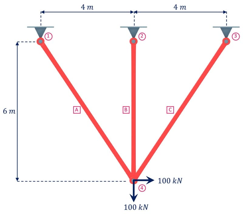
Fig. 2. Simple 3-bar plane truss
Our first task is to identify each possible displacement, ignoring the influence of supports (for now), each node could undergo two orthogonal displacements, Fig.
- We’ll call these degrees of freedom, our structure therefore has 8 degrees of freedom. This will come up again later when we’re building the primary structure stiffness matrix.
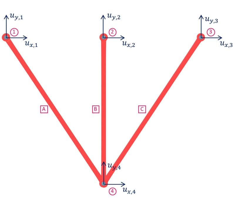
Fig. 3. Degrees of freedom
3.1 Global Element Stiffness Matrix
In order to combine our element stiffness matrices together, we must first account for the fact that they are all orientated at different angles. This means that an axial force for member A for example cannot currently be directly added to an axial for from member B as they are orientated at different angles. So we need to perform a transformation that maps forces and displacements from each member into a common global reference frame. For this we use a transformation matrix, . Now this can be easily derived but in the interest of brevity, for now we simply state the following relationship between coordinates in a local member reference frame and the corresponding coordinates in a global structure reference frame,
where and are the local axial displacements at nodes 1 and 2. We can summarise this as . The transformation matrix acts as a bridge between local and global coordinates provided we use a method of determining the angle of orientation of the member in question, , and stick to it for all members. We can use the exact same technique to bridge between forces in a local element reference frame and their values in the common (to all members) global reference frame.
Again it will help us to summarise this relationship as . Now that we have the link between:
- forces in a local and global reference frame
- displacements in a local and global reference frame
we need to finally link up forces in a global reference frame with displacements in a global reference frame. Trust me, this is going somewhere! Consider equation (7) that relates local element force and displacement,
We can substitute this equation into equation (9), replacing to get,
Now using equation (8) to replace yields,
Therefore we can identify as the Global Element Stiffness Matrix, that relates forces defined in a global reference frame to displacements also defined in a global reference frame. For clarity, let’s now define and . After performing the matrix multiplication, , we obtain as,
Now we can calculate a global element stiffness matrix for each element in our structure that encodes the orientation of the member. Once calculated, these can then be directly combined to build the primary structure stiffness matrix.
3.2 Element A – Global Element Stiffness Matrix
Consider element A, Fig. 4. Note that the degrees of freedom at nodes 1 and 4 are shown in the local element reference frame.
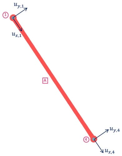
Fig. 4. Element A showing degrees of freedom in a local reference frame
For a member between nodes and , we define the angle of orientation, as the angle (in radians) measured counter-clockwise between the positive global x-axis and the local x-axis, with node at the origin where . In this case, that makes radians . Noting that element A is long, we can use equation 13 to obtain the global element stiffness matrix,
3.3 Element B – Global Element Stiffness Matrix
For element B, Fig. 5, we have radians . With a length of m, we have,
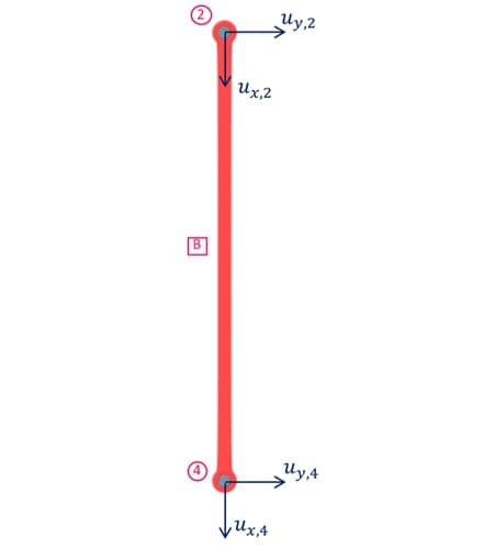
Fig. 5. Element B showing degrees of freedom in a local reference frame
3.4 Element C – Global Element Stiffness Matrix
Element C, Fig. 6, has an angle of orientation radians and length of m. This gives us a global element stiffness matrix of,
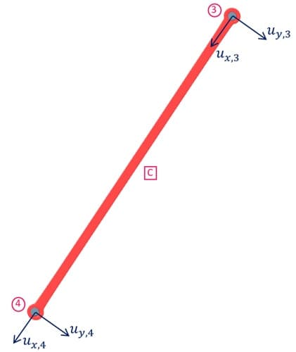
Fig. 6. Element C showing degrees of freedom in a local reference frame
3.5 Building the Primary Structure Stiffness Matrix
Next we’ll work our way through building the primary structure stiffness matrix. This is usually the part of the process most prone to error so we’ll approach it in a methodical step-by-step fashion to cut down the likelihood of errors.
Step 1: Break the element stiffness matrices into quadrants
Each element stiffness matrix is , so we’ll break each one up into quadrants. So element A for example would be divided as follows,
where,
The same subdivision process is repeated for each member of our structure.
Step 2: Set up the primary stiffness matrix template
Now we can set up a template for the primary stiffness matrix that will make it easy to see where the quadrants of our element stiffness matrices slot in. Since our structure has 4 nodes, our template will be , for now we can fill it with placeholders as follows,
Each element in the template above actually represents a matrix, so this template actually represents an primary structure stiffness matrix, when filled in.
Step 3: Fill in the template with the quadrants of the element stiffness matrices
Now we can take the quadrants of the element stiffness matrices and slot them into the relevant positions in the primary stiffness matrix template. For each member, identify the node numbers at each end of the member, this defines the rows and columns into which that member’s quadrants fit. More specifically, the quadrants of the element stiffness matrix are positioned at the intersection of the rows and columns identified by the node numbers. Consider member A as an example; it joins nodes 1 and 4, and so it contributes to the primary stiffness matrix as follows,
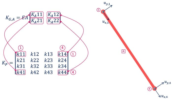
Fig. 7. Contribution of element A to the primary stiffness matrix template
We follow the exact same process to add all of the element stiffness matrices into the primary stiffness matrix. Notice that every time we add the contribution from another member, we end up adding to element . Based on our earlier discussion of the direct stiffness method concept, this makes sense as all members meet at node 4 and therefore contribute to the behaviour of that node. We can see how the primary stiffness matrix evolves with the addition of each member. After adding element A, we have,
Notice that the matrix is full of zeros, except for the quadrants (four corners) associated with nodes 1 and 4. After adding element B we obtain,
Finally after adding element C we have the full primary element stiffness matrix. This matrix is essentially our structural model and the link between force and displacement for the entire structure,
3.6 Imposing Boundary Conditions on our Model
At this stage it’s worth taking stock of where we are; we’ve fully modelled the force displacement relationship for our structure and we effectively have the hard work done. Now it’s just a matter of crunching the numbers to solve for our deflections, reactions and member forces.
Taking another look at our problem, we note that we have 14 variables which consist of 8 degrees of freedom/displacements and 6 reactions. But we haven’t taken into consideration yet the fact that 6 of our degrees of freedom are constrained to be zero by our supports, i.e. degree of freedom 1, 2, 3, 4, 5, and 6 are fully restrained by pin supports at nodes 1, 2 and 3. As a result, we actually only have 14-6 = 8 unknowns to solve for. This ties up nicely with the fact that we have a system of 8 simultaneous equations we can use to identify our unknowns. Our system of 8 simultaneous equations is as follows,
Before we try and solve this system of equations, we have one more issue to take care of. We need to impose the known displacements onto our system of equations. Again, we do this in quite a systematic way by placing 1 in the diagonal corresponding to known zero displacement and 0 in all other elements of corresponding rows and columns of the primary stiffness matrix. We also place 0 in the corresponding elements of the force vector. So in our case, considering the and displacement for nodes 1, 2 and 3, (corresponding to degrees of freedom – ) are zero, our system of equations becomes,
We define this ‘reduced’ stiffness matrix, the Structure Stiffness Matrix, , dropping the ‘primary’ to differentiate it from the original primary stiffness matrix. We can see that placing zeros in the primary stiffness matrix rows imposes the boundary conditions,
While placing zeros in the primary stiffness matrix columns ensures known displacements remain zero in subsequent calculations, e.g. consider row 7,
After our boundary conditions are imposed, we can condense our system of equations and substitute in values for the forces at node 4,
We can then solve this system of 2 simultaneous equations by inverting the structure stiffness matrix,
Note that the horizontal displacement is positive, indicating that it acts to the right, according to our global axis system. Similarly the negative value for vertical displacement indicates a downward pointing displacement.
Remember that these are the values of displacement that simultaneously satisfy the force-displacement model for each member that connects into node 4. It’s also worth noting that at no point did the fact that the truss us statically indeterminate feature in our discussion. This is one of the great advantages that this analysis technique has over other analysis methods that rely on equations of equilibrium (method of sections and joint resolution). Before we can call this analysis complete, we need to work out our reactions and internal member forces.
3.7 Calculating Reactions
Calculating reactions is simply a matter of substituting our known displacements back into our full structural model, i.e. the force-displacement relationship that uses the primary structure stiffness matrix,
From this we directly obtain the vector of forces which contain the reactions,
At this stage, it’s helpful to visualise these on the structure, Fig. 8.
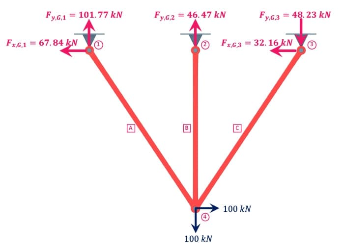
Fig. 8. Truss reactions
3.8 Solving for Truss Member Forces
In order to solve for the internal axial force in each member, we return back to where it all began…recall equation 1,
To be a little more precise, we can say that the force in the element between nodes and is given by,
This requires us to convert our calculated global displacements at node and back into local displacements measured in the local element reference frame using our transformation matrix from above.
So for element A with radians, we have,
Using these displacements in equation 36, we obtain the axial force in element A,
We can repeat the exact same process for elements B and C to obtain their axial forces as and respectively. The negative sign here indicating compression rather than tension in the element.
That more or less wraps up our example analysis – we’ve solved for all unknown displacements, reactions and member forces. As a final task, we can substitute in values for Young’s modulus and cross-sectional area . Doing this we obtain the following deflections for node 4 (obviously the reactions and member forces are unchanged) ,
We can visualise these results below, Fig. 9.
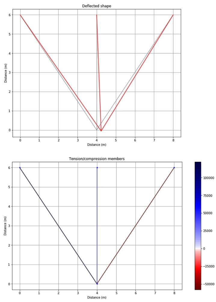
Fig. 9. (Top) Deflected shape with magnification. (Bottom) Axial force diagram in which reds indicate compression and blues indicate tension. Produced using codes from The Direct Stiffness Method for Truss Analysis with Python online course.
ONLINE TRUSS TOOLBOX 🛠️
Try our free truss analysis toolbox for calculating reactions, axial forces and deflections. A handy tools for students and professional engineers.
3.9 Implementing the Direct Stiffness Method in Practice
As you can see, once we nail down the basic underlying principles, the direct stiffness method really is quite a simple analysis technique. You might also have recognised the one major bottleneck with this approach…inverting the structure stiffness matrix. In our example, this was a matrix, relatively trivial to invert. But as the number of nodes in our structure increases, so too does the size of the matrix we need to invert. We very quickly reach a point where we need to resort to computers to do the computational heavy lifting.
The upside here is that once we implement the solution process in an algorithm, the task of solving structures we wouldn’t even consider by hand, becomes quick and easy! You essentially implement your own structural analysis software. The 3D transmission tower, Fig. 10. is analysed using the same methods we discussed above. It’s really only when we implement the direct stiffness method in an algorithm that its power and scalability really shine through.
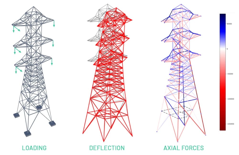
Fig. 10. Three dimensional model of a transmission tower analysed using the direct stiffness method. This analysis is an extract from the online course 3D Space Frame Analysis using Python and Blender.
4.0 Implementing the Direct Stiffness Method – Where to Next?
Now that you understand conceptually how the direct stiffness method works, why not build on this and build a practical implementation. In the three EngineeringSkills courses in our Direct Stiffness Method Course Bundle, we work our way through building out a complete suite of analysis codes using Python (if you’re new to Python – no problem!). We start with with 2D plane trusses, then move on to beam and frame structures that experience bending and shear before expanding into full 3D space frame structures. After completing this suite of courses you’ll have the knowledge and practical tools to analyse a huge range of structures without resorting to commercial structural analysis software. And if you do use commercial software, you’ll understand exactly how it’s working behind the scenes.
Dr Seán Carroll's latest courses.


Featured Tutorials and Guides
If you found this tutorial helpful, you might enjoy some of these other tutorials.
Arch Analysis – How to Analyse Determinate and Indeterminate Arches
Learn how to apply virtual work methods to unlock the behaviour of indeterminate arches

Callum Wilson
