Machine Learning in Civil Engineering - Sensitivity Analysis
![[object Object]](/_next/image?url=%2Fimages%2Fauthors%2Fehsan_eshaghi.jpg&w=256&q=75)

Welcome to our first tutorial on machine learning in civil engineering! In this series, Ehsan Es'haghi will explore how machine learning can be used to solve complex engineering problems.
We'll start by learning how to define a simple optimisation objective function, such as minimising compliance in a structure. From there, we'll explore the concept of sensitivity analysis and its crucial role in optimisation problems. Then, we’ll focus on the adjoint method, a clever and widely used technique in industrial optimisation software. To tie everything together, we'll implement these concepts from scratch in Python, working through an example where we iteratively modify the size of elements in a truss structure.
By the end of this tutorial, you'll have a solid understanding of sensitivity analysis and be ready to tackle more advanced topics in machine learning and structural optimisation.
📂 Make sure to download the Jupyter Notebook (linked above) to run locally as you read through the tutorial.
Now, over to Ehsan!

In this tutorial, our goal is to redistribute a fixed amount of material among the elements of a truss in order to minimise the total deformation of the structure.
Our case-study structure for this exercise is the 2D truss shown in Fig 1. below. For the purpose of this discussion, let’s assume that of steel has been used to construct the truss.
Essentially, by removing some elements and increasing the size of others, we can reduce the deformation while maintaining the same overall weight. Our task now is to establish a systematic way of achieving this goal.
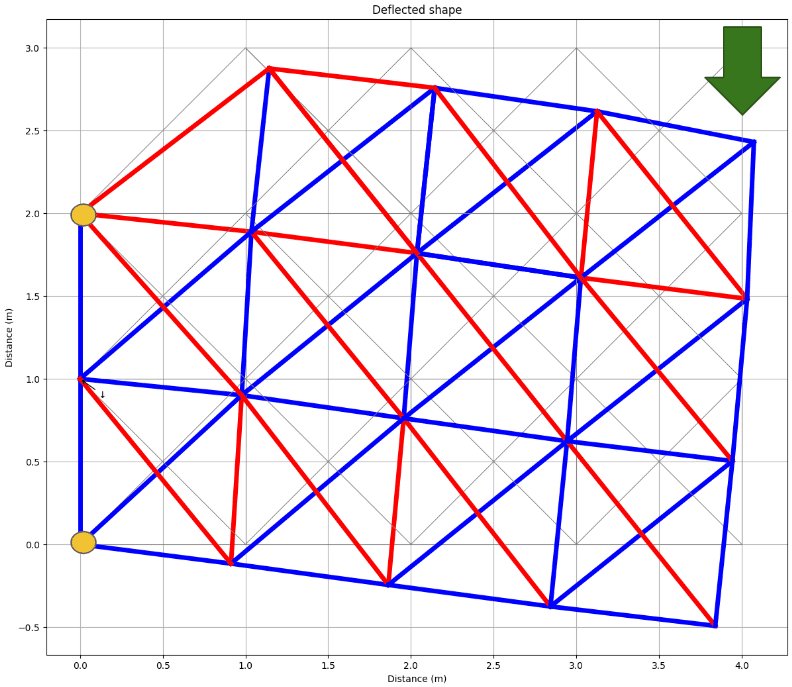
Fig 1. Case-study 2D truss consisting of a fixed quantity of steel ().
1.0 The constrained optimisation problem
In the field of layout optimisation, global compliance is a commonly used optimisation objective. It refers to the sum of the work done on the structure's nodes and is equivalent to the total strain energy stored in the structure.
This measure reflects the structure's flexibility; thus, minimising compliance ensures the structure is as stiff as possible, reducing deformations under load and enhancing structural performance.
Mathematically, in terms of the applied force vector , the stiffness matrix , and the displacement vector , the compliance is given by:
Our aim is to solve the following constrained optimisation problem:
Minimise by modifying the size of the elements
subject to: the weight of the structure remaining
where:
Note that and are vectors, so their dot product is given by,
which represents the total work done on the structure's nodes by the external force.
In this specific example (Fig. 1), the external force is constant and applied only at one node, making global compliance dependent solely on the displacement of that node. Therefore, we seek a truss structure that minimises the displacement of the upper right node.
Given , the displacement vector can be derived by solving the system of linear equations involving the stiffness matrix and the force vector .
1.1 Sensitivity of global compliance
To redistribute material by removing some elements and reallocating their mass to others, we need to rank the elements based on their contribution to compliance minimisation (minimising the displacement of the upper right node in this specific problem).
The naive approach is to remove the element with the least impact on compliance and distribute its mass among the remaining elements.
However, to determine this ranking, we need to perturb the size of each element and measure the resulting change in node displacement. This defines the sensitivity of global compliance to the size of each element, which is essentially the derivative of compliance with respect to the size of each element.
We repeat this process iteratively until no further reduction in global compliance can be achieved by removing another element. This procedure is an iterative optimisation algorithm, depicted in the following flowchart.
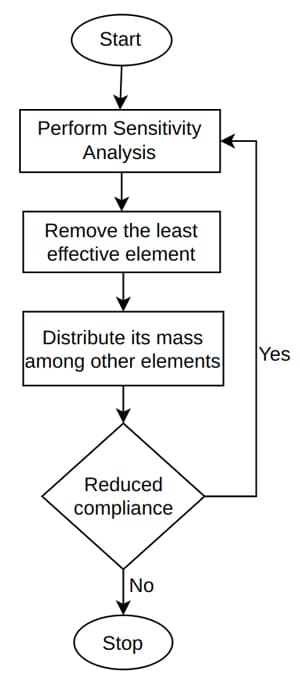
Fig 2. Flowchart showing the iterative optimisation algorithm.
Performing sensitivity analysis can be computationally intensive. In the next section, we will delve into the mathematical formulation of global compliance and sensitivity analysis to better understand the complexity of this problem.
We will introduce and compare various approaches for sensitivity analysis, evaluating their complexities. Subsequently, we will implement an efficient sensitivity analysis approach and the algorithm outlined in the flowchart.
Although these methods have been demonstrated with a simple case-study, they are extensively applied in industry. For further insights, consider exploring products built on similar principles from Autodesk and Altair.
2.0 Sensitivity Analysis for Stiffness Maximisation
In a scenario where the variable of interest is the size of the truss elements, the goal is to minimise compliance by optimally adjusting the size of each element, which in turn modifies the stiffness matrix .
Let’s denote the size parameter of each truss element by . The task is to compute the sensitivity of the compliance with respect to each size parameter . This can be expressed as:
We can easily see that,
because .
However, to compute , we need to consider the implicit relationship through the stiffness matrix . More specifically, since is not given explicitly but is the solution of the equation , we have implicitly in the form . This implicit relationship makes it challenging to directly calculate the derivative of with respect to .
The computational complexity of this problem is , where is the number of nodes and is the number of elements (or edges) whose sizes we are optimising.
Solving the linear system of equations with N equations and N unknowns is computationally expensive, with a complexity of . If we want to optimise the size of elements in our structure to minimise compliance, we need to perform this computation times, each time computing the impact of one element's size on the compliance of the structure.
Afterwards, we can increase the size of elements with the largest magnitude of the gradient and decrease the size of elements with a small gradient magnitude to decrease compliance while keeping the weight of the structure almost constant. We can repeat this process multiple times to find a -dimensional vector that minimises compliance.
2.1 Finite Difference Method and Its Computational Cost
The finite difference method is a straightforward approach to compute the sensitivity of the compliance. It involves perturbing each design variable by a small amount and observing the resulting change in compliance. The sensitivity is then approximated by:
While easy to implement, this method is computationally expensive, especially for large-scale problems with many design variables. Each perturbation requires solving a new system of equations, leading to a high computational cost.
2.2 Gradient Descent Method
To understand the iterative optimisation process, it is essential to have a brief understanding of gradient descent. Gradient descent is an optimisation algorithm used to minimise a function by iteratively moving in the direction of the steepest descent, as defined by the negative of the gradient. In each iteration, the parameters are updated using the formula:
where is the learning rate, a positive scalar determining the step size.
In our context, this means we adjust the sizes of the truss elements iteratively, guided by the gradients of compliance with respect to the size parameters.
By continuously updating the parameters in the direction that reduces compliance, we aim to find an optimal configuration that maximises the stiffness of the structure.
2.3 Efficiency with the Adjoint State Method
The adjoint state method provides a more efficient way to compute the sensitivity of compliance. Instead of perturbing each design variable independently, this method involves solving an additional system of equations— the adjoint equations.
The adjoint method leverages the solution of the primal system (original equations) to compute the sensitivities more efficiently. Without proof, the adjoint equation is given by:
where is called the adjoint vector.
The complete adjoint solution proof is provided at the end of this tutorial for interested readers.
The sensitivity of the compliance with respect to the design variable can then be computed as:
By solving the adjoint equation once, the sensitivities with respect to all design variables can be obtained, significantly reducing the computational cost compared to the finite difference method.
Please note that is an -dimensional matrix because we are taking the derivative of an -dimensional matrix with respect to a -dimensional vector. Therefore, you need to take the derivative of times, each time with respect to the size of one element, then concatenate them to obtain the full matrix.
Recall the stiffness matrix for a truss, which is defined as follows:
Taking the derivative of with respect to each element size is straightforward by removing :
Please also note that we used as a vector of element sizes, so size of the -th element.
In addition, in relation to the code below, it's worth mentioning that the Numpy command np.linalg.solve(A, b) should generally yield the same result as np.matmul(np.linalg.inv(A), b). However, the former approach is preferred because, although not proven here, explicitly computing the inverse of a matrix can be numerically unstable. Therefore, it is usually best to avoid taking the inverse directly in your code.
3.0 Implementing the adjoint method
Now we’ll implement the adjoint method. This will require us to implement the direct stiffness method for 2D truss analysis. To achieve this and streamline the discussion, we’ll define many utility functions. For brevity, they’re simply listed below, but the body of these functions can be found in the utils.py file as part of the downloadable resources for this tutorial.
Remember, the complete optimisation process can be observed and studied by running the associated Jupyter Notebook, linked above. You’re encouraged to study this tutorial and the Jupyter Notebook, in parallel.
The following utility functions are defined; their purpose is evident from the function names. If you’re not familiar with the implementation of the direct stiffness method for 2D truss analysis (integral to this implementation), you should review the EngineeringSkills course The Direct Stiffness Method for Truss Analysis with Python.
The Direct Stiffness Method for Truss Analysis with Python
Build your own finite element truss analysis software using Python and tackle large scale structures.
After completing this course...
- You’ll understand how to use the Direct Stiffness Method to build complete structural models that can be solved using Python.
- You’ll have your own analysis programme to identify displacements, reactions and internal member forces for any truss.
- You’ll understand how common models of elastic behaviour such as plane stress and plane strain apply to real-world structures.
def member_rotation(member, nodes):
	# Calculate the orientation and length of a single member

def calc_rotation_length(members, nodes):
	# Calculate the orientation and length of all members by calling member_rotation()

def plot_deflection(members,nodes,mbrForces,members_area,UG,xFac,turn):
	#Plot the deflected shape of the structure

def calc_member_forces_def(member,A,theta,L,U,E):
	# Calculate the member forces based on deflection

def build_matrix_reduced(matrix, restrained_DOF):
	# Build the 'structure' stiffness matrix

def calc_displacement(K, force_vector, restrained_DOF):
	# Solve the system of equations to determine the nodal displacement vector

def assemble_UG(U, n_DOF, restrained_DOF):
	# Construct the global displacement vector

def calculate_Kg(theta,mag,E,A):
	# Calculate the global stiffness matrix for an axially loaded bar

def calc_DOF(members):
	# Calculate the number of degrees of freedom in the structure

def build_K(members, members_area, orientations, lengths, E):
	# Build the primary stiffness matrix for the structure
Next, we define a class to represent the structure and contain variables and methods associated with it. This class and its member functions will call various of the utility functions defined above. Note that this class assumes that we have the following .csv files located in a folder called initial_structure:
members.csv→ contains the node numbers defining each membernodes.csv→ contains the x/y coordinates of each nodesupports.csv→ contains a list of restrained degrees of freedom
The StructEnvironment() class is defined as follows:
class StructEnvironment():
    def __init__(self):

        # Constants
        self.E = 200 * 10**6  # (N/m^2) Young's modulus
        self.nodes = np.genfromtxt('initial_structure/nodes.csv',delimiter=',',dtype=np.float16)
        self.step_size = 0.01
        self.A = 0.01  # default size of element

        # Supports
        self.restrained_DOF = np.genfromtxt('initial_structure/support.csv',delimiter=',',dtype=np.int8)

        # Members
        self.members = np.genfromtxt('initial_structure/members.csv',delimiter=',',dtype=np.int8)
        self.DOF = calc_DOF(self.members)
        self.element_count = len(self.members)

        # Loading
        self.point_loads = np.array([np.zeros(self.DOF)]).T.ravel()
        self.point_loads[36] = -100*1e3
        self.point_loads[37] = -100*1e3

        # Define any additional environment-specific variables here
        self.current_step = 0
        self.rotations, self.lengths = calc_rotation_length(self.members, self.nodes)

        # Constraint
        self.total_area = sum(self.A*self.lengths)

    def analyse(self,members_area):
        K = build_K(self.members, members_area, self.rotations, self.lengths, self.E)
        del_K__del_area = build_del_K__del_area(self.members, members_area, self.rotations, self.lengths, self.E)
        U_free = calc_displacement(K, self.point_loads, self.restrained_DOF)
        UG = assemble_UG(U_free, self.DOF, self.restrained_DOF)
        U_2d = UG.reshape((-1,2))
        self.deflections = []
        def_members = np.zeros((self.element_count))
        F_members = np.zeros((self.element_count))
        for i in range(self.element_count):
            L = self.lengths[i]
            F_member,def_member =  calc_member_forces_def(self.members[i],members_area[i],self.rotations[i],L,U_2d,self.E)
            def_members[i] = def_member/L
            F_members[i] = F_member
        return F_members,def_members,UG,del_K__del_area,K

    def calculate_cost(self,UG): # global compliance
        return UG@self.point_loads

    def reset(self):
        self.current_step +=1
        members_area = np.random.normal(loc=self.A,scale=self.A/3,size=len(self.members))
        members_area[members_area<1e-4] = 1e-4
        members_area = self.redistribute_material(members_area)
        return members_area

    def redistribute_material(self,members_area):
        members_area = members_area * (self.total_area/sum(members_area*self.lengths))
        return members_area

    def update_area(self,members_area):
        random_element = np.random.randint(self.element_count)
        members_area[random_element] = members_area[random_element] + np.random.normal(loc=0,scale=self.A/5)
        members_area[members_area<1e-4] = 1e-4
        members_area = self.redistribute_material(members_area)
        return members_area

    def step(self, members_area):
        F_members,def_members,UG,del_K__del_area = self.analyse(members_area)
        cost = self.calculate_cost(def_members)
        return cost,F_members,UG

    def render(self,members_area,F_members,UG):
        plot_deflection(self.members, self.nodes,F_members, members_area,UG ,2,self.current_step)
3.1 Adjoint Method (Sensitivity Analysis)
Before implementing the iterative sensitivity analysis, we define the following 3 additional helper functions required to calculate the sensitivity:
def calculate_del_Kg__del_area(theta,mag,E,A):

    c = math.cos(theta)
    s = math.sin(theta)

    K11 = (E/mag)*np.array([[c**2,c*s],[c*s,s**2]]) #Top left quadrant of del_Kg__del_area
    K12 = (E/mag)*np.array([[-c**2,-c*s],[-c*s,-s**2]]) #Top right quadrant of del_Kg__del_area
    K21 = (E/mag)*np.array([[-c**2,-c*s],[-c*s,-s**2]]) #Bottom left quadrant of del_Kg__del_area
    K22 = (E/mag)*np.array([[c**2,c*s],[c*s,s**2]]) #Bottom right quadrant of del_Kg__del_area
def build_del_K__del_area(members, members_area, orientations, lengths, E):
    n_DOF = calc_DOF(members)
    Kp = np.zeros([n_DOF, n_DOF])  # Initialise the primary stiffness matrix
    d_Kp__d_area = np.zeros((n_DOF, n_DOF,len(members)))
    for dimension in range(len(members)):
        for n, mbr in enumerate(members):
            # note that enumerate adds a counter to an iterable (n)

            # Calculate the quadrants of the global stiffness matrix for the member
            theta = orientations[n]
            L = lengths[n]
            A = members_area[n]
            if n == dimension:
                [K11, K12, K21, K22] = calculate_del_Kg__del_area(theta, L, E, A)
            else:
                continue

            node_i = mbr[0]  # Node number for node i of this member
            node_j = mbr[1]  # Node number for node j of this member

            # Primary stiffness matrix indices associated with each node

            i = 2* node_i
            j = 2 * node_j

            d_Kp__d_area[i : i + 2, i : i + 2,dimension] = Kp[i : i + 2, i : i + 2] + K11
            d_Kp__d_area[j : j + 2, j : j + 2,dimension] = Kp[j : j + 2, j : j + 2] + K22
            d_Kp__d_area[i : i + 2, j : j + 2,dimension] = Kp[i : i + 2, j : j + 2] + K12
            d_Kp__d_area[j : j + 2, i : i + 2,dimension] = Kp[j : j + 2, i : i + 2] + K21

    return d_Kp__d_area
def gradient(K,F,U,del_K__del_area,A,lengths,C,restrained_DOF):
    K_reduced = build_matrix_reduced(K,restrained_DOF)
    del_K_reduced__del_area = build_matrix_reduced(del_K__del_area,restrained_DOF)
    F_reduced = build_matrix_reduced(F,restrained_DOF)
    U_reduced = build_matrix_reduced(U,restrained_DOF)

    lambda_ = np.linalg.solve(K_reduced.T,F_reduced.T) # solving adjoint equation
    d_L__d_area = np.zeros((len(F),len(lengths))) # ( N, P)
    temp = np.zeros((len(U_reduced),len(lengths)))
    for i in range(len(lengths)):
        temp[:,i] = del_K_reduced__del_area[:,:,i]@U_reduced # d_k/d_theta * U

    d_L__d_area =  - lambda_.T @ temp # - lambda * d_k/d_theta * U
    return d_L__d_area
Iterative Analysis
In the following code, during each iteration, we find the element with the minimum gradient value, specifically the minimum magnitude of the gradient, since all the gradients are negative. Why is this the case? Because increasing the size of any element will cause the compliance to decrease.
Our goal is to find the element whose size change has the least impact on compliance. We then remove this element and redistribute its material to other elements.
However, we do not actually remove an element, as this could make our structure indeterminate, preventing analysis using the direct stiffness matrix and requiring the use of dynamic equations, which is beyond the scope of this tutorial. Instead, we reduce the size of the element to a value very close to zero .
This approach is called a greedy algorithm because, at each step, we greedily remove the element with the minimum gradient magnitude. It is worth mentioning that while the greedy algorithm quickly finds a good structure, it does not guaranteed to be the optimal structure in terms of compliance.
In other words, if we had the time to compute the compliance for all possible combinations of elements, there might be a combination that results in less compliance than what we find using this greedy algorithm.
To clarify further, note that when we decide to remove an element in one iteration due to its small gradient, the gradient of that element might become significant in subsequent iterations.
In other words, an element might not be resisting load in one iteration, but after the structure is modified, it could come under a significant load. However, our code keeps track of removed elements and ensures that material is not added to removed elements in any subsequent iterations, thereby keeping them removed.
env = StructEnvironment()
cost = []

members_area = env.reset()
members_area = np.ones_like(members_area) * env.A

removed_indices = []
i = 0
while True:
    F_members,def_members,UG,del_K__del_area,K = env.analyse(members_area) # del_K__del_area.shape = N*N*P
    new_cost = env.calculate_cost(UG)
    if (len(cost)>0) and (new_cost > 5*cost[i-1]):
        break
    cost.append(new_cost)

    env.render(members_area,F_members,UG)
    gradient_area = gradient(K,env.point_loads,UG,del_K__del_area,members_area,env.lengths,env.total_area,env.restrained_DOF)
    edges_sorted_by_importance = np.argsort(gradient_area)[::-1]
    j = 0
    while True:
        if edges_sorted_by_importance[j] not in removed_indices:
            removed_indices.append(edges_sorted_by_importance[j])
            break
        j +=1

    print(f"iteration: {i} , cost: {cost[i]}") # cost is the same as compliance : F.T @ U
    members_area[np.array(removed_indices)] = 1e-4 # set size of the removed elements very close to 0
    members_area = env.redistribute_material(members_area) # redistribute the material among the elements which are not removed
    env.current_step +=1
    i += 1

cost = np.array(cost)
This code iterates until there is no further appreciable reduction in compliance. By calling render() on each iteration we can observe how the structure evolves as the material is progressively redistributed throughout the structure. This results in over 40 plots of the structure, which we obviously won’t show here (run the code yourself to see this). Noting that the initial state of the structure is shown in Fig 1. above, we can see the final structural configuration in Fig 3. below.
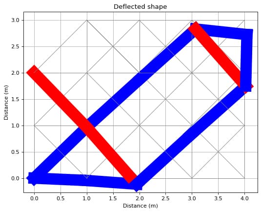
Fig 3. Optimised structure that minimises deflection under the point load by redistributing mass throughout the structure. Note red members are in tension and compression members are shown in blue.
We can plot the cost versus global compliance to observe the rate at which convergence was obtained, Fig 4.
plt.plot(cost)
plt.xlabel('iteration')
plt.ylabel('cost')
plt.title('Cost : global compliance')
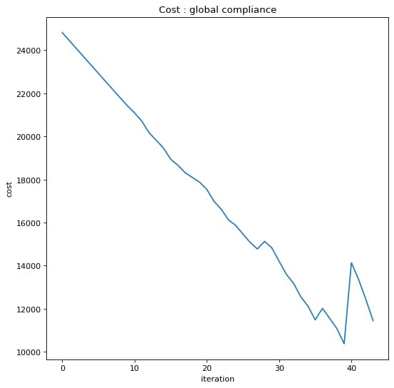
Fig 4. Plot showing cost versus global compliance.
We encourage you to try to implement the same algorithm using the finite difference method, and compare your results with this code, in terms of compliance reduction rate, and running time.
In our next tutorial on machine learning in Civil Engineering, we’ll explore how surrogate models can be used to approximate structural behaviour and deliver results significantly faster than traditional analysis techniques.
Given , where is dependent on the size of the element, we denote the vector of element sizes as , which has dimensions . Our objective is dependent on , and is dependent on . Therefore, we have:
To find :
Since is not directly dependent on :
Given :
To derive :
Since :
Given that because the external force is given and not dependent on :
Substituting into :
or is the solution of .
Please, pay attention that is an matrix (with rows and columns). In other words, in order to compute , you need to run , times for . Each iteration has computational cost. Then you need to stack those columns to get and finally multiply by to find . I hope you can observe that this algorithm has computational cost.
Now, let's consider the adjoint bracketing trick:
Let . You can solve for by running which has complexity. After computing , we can compute the derivative as follows:
Therefore, instead of computing times (once for each element), we calculate once and then multiply it by , which is an tensor. The adjoint method is essentially a clever bracketing that reduces the computational complexity of the gradient from to .
Here is our algorithm:
- Compute in .
- Compute in .
- Compute in , since it's just a matrix-vector multiplication.
Since is much less than , we can ignore that part and conclude that we have an algorithm that computes the derivative of global compliance with respect to all size parameters in .
If you're interested in learning more about the Adjoint method, I highly recommend checking out this playlist. It's where I first learned about it myself.
-
Some of the utility functions are adapted from The Direct Stiffness Method for Truss Analysis Course from EngineeringSkills.com
-
Adjoint method codes are adapted from Automatic Differentiation, Adjoints & Sensitivities Playlist on Youtube
Featured Tutorials and Guides
If you found this tutorial helpful, you might enjoy some of these other tutorials.

Machine Learning in Civil Engineering - Surrogate Models
Part 2 - Explore the predictive power and computational efficiency of Surrogate Models

Ehsan Es'haghi

How to Calculate Beam Deflection
How to calculate beam deflection from first principles, with calculation examples

Dr Seán Carroll