Shear and Moment Diagrams – An Ultimate Guide
![[object Object]](/_next/image?url=%2Fimages%2Fauthors%2Fsean_carroll.png&w=256&q=75)

In this tutorial, we're going to take a look at shear and moment diagrams in detail. Determining shear and moment diagrams is an essential skill for any engineer.
In my experience teaching undergraduate engineering students, it's probably the one structural analysis skill they struggle with most.
Not being able to reliably draw shear and moment diagrams is a problem! You can't complete a design without understanding how shear forces and bending moments are developed in a structure. Shear force and bending moment diagrams tell us about the underlying state of stress in the structure. So naturally, they're the starting point in any design process.
Another reason every graduating engineer needs to have a solid grasp of shear forces and bending moments is that they're absolutely going to be tested in almost every graduate interview.
The quickest way to tell a great CV writer from a great graduate engineer is to ask them to sketch a qualitative shear and moment diagram for a given structure and load combination.
Don’t get caught out!
This tutorial will be a thorough, one-stop-shop introduction to shear forces, bending moments and how to draw shear and moment diagrams. By the time you work your way through this deep dive, you’ll have a solid understanding of how to construct shear and moment diagrams for statically determinate beam and frame structures.
I’ve tried to make this tutorial a complete course in constructing shear and moment diagrams, so take your time working through it. There are no prizes for finishing quickly!
We have a lot of ground to cover! So, we’ll break our study of shear forces and bending moments up as follows:
📍 1.0 The Basics - What are Shear Forces and Bending Moments
You’re probably here because you just want to know how to go from a loading diagram to a shear and moment diagram...as quickly as possible! We’ll definitely get to that...but it will serve us well to start by clearing understanding what exactly the shear and moment diagram are actually telling us.
📍 2.0 Calculating Internal Shear Forces and Bending Moments
With the basics covered, we’ll move on to calculating shear forces and bending moments at discrete locations in the structure. This gives us the ability to ‘open up the structure’ and any point and determine discrete values of shear and moment - a powerful tool!
📍 3.0 Building Shear and Moment Diagrams
Discrete values of shear and moment are great, but it’s a full diagram we’re after! To construct the shear and moment diagrams we need to determine expressions for how the shear and moment change throughout the structure. Plotting these expressions gives us our diagrams. We’ll cover this in section 3.
📍 4.0 Shear and Moment Diagram - Beam Example Walkthrough
In section 4, we’ll work through a beam example, building the shear and moment diagram, step-by-step, using what we’ve learned so far. I encourage you to continue reading the complete tutorial. But, I've also recorded full video walkthrough solutions for each example. I suggest watching these once you've finished reading through the tutorial.
This section is where we establish the procedure or workflow that we’ll follow in all future examples. Half of structural analysis is just ensuring you meticulously follow your procedures - so pay special attention to the steps we take here.
📍 5.0 Digging Deeper - Relating Loading, Shear Force and Bending Moment
Up to this point, our workflow has been very mechanical—we follow a sequence of steps that always lead to the right result. But have you ever wondered how some engineers can look at a structure and simply state what the shear force and bending moment diagram will look like without doing any calculations?
This is possible when you understand some fundamental relationships between loading, shear force, and bending moment. We’ll cover this next, and it will dramatically improve your intuition for shear and moment diagrams.
📍 6.0 Shear and Moment Diagram - Beam Example Walkthrough 2
After we’ve gained a deeper understanding of the link between loading, shear force and bending moment in the previous section, we’ll put this to the test with another beam analysis walkthrough. This time we’ll also take the opportunity to introduce another new detail - hinges!
📍 7.0 Shear and Moment Diagram - 2D Frames
By this point, you’ll have no problem tackling beams - but what about 2D frame structures? It’s not that difficult to bolt on a couple of extra ideas and expand what we know to frames. So, this is what we’ll cover in section 7. Since we have the core theory covered already, we can tackle frames directly by working through an example.
📍 8.0 What Comes Next - More Resources and Other Techniques
Mastering any structural analysis technique is all about practice! So, in this section, I’ll point you towards some additional EngineeringSkills resources that will give you more questions to work on and compare your answers to - students get free access to these resources :)
This tutorial focuses on statically determinate beam and frame structures—this just means we can use the three equations of statics to solve for the reactions (and complete the shear and moment analysis). For statically indeterminate structures, we need to employ some fancier techniques. I’ll point to those EngineeringSkills resources in this final wrap-up section.
Many of these resources are also completely free for students.
Finally, if you want to sprinkle some Python over your new shear and moment diagram skills and build tools to do the analysis for you, I’ll point to those references, too.
1.0 The Basics - What are Shear Forces and Bending Moments
Shear forces and bending moments are what we call stress resultants. This simply means they are the force and moment that result from the shearing and normal stress (due to bending) at a section in the structure.
This is useful because if we can use the externally applied forces to calculate a shear force and bending moment, we can work backwards to get the corresponding stresses in the structure. Once we know the stresses induced by some external loading, we can design for that loading by ensuring the stresses can be accommodated by the structural material.
Now, let’s take a closer look at the bending moments and shear forces and how they relate to stresses.
1.1 What is a Bending Moment?
Let’s start with a basic question; what is a bending moment? To answer this we need to consider what’s happening internally in a structure under load. Consider a simply supported beam subject to a uniformly distorted load, Fig 1.

Fig 1. Simply supported beam subject to a uniformly distributed load (top), deformed beam showing the change in length of longitudinal fibres (bottom). Note that the arrow directions indicate the direction of internal stress and not the elongation direction of fibres (opposite).
In order for the beam to deflect as shown, the fibres in the top of the beam must get shorter while the fibres in the bottom of the beam must get longer.
We can say the top of the beam is in compression while the bottom is in tension (notice the direction of the arrows on the fibres in the deflected beam). Now, at some position in the depth of the beam, compression must turn into tension. There is a plane in the beam where this transition between tension and compression occurs. This plane is called the neutral plane or sometimes the neutral axis.
The neutral plane is a plane at some point in the depth of the beam where the length of longitudinal fibres remains unchanged.
Imagine taking a vertical cut through the beam at some distance along the beam. In doing so, we can imagine revealing the internal strain and stress distributions throughout the depth of the beam, Fig 2.

Fig 2. Strain and stress distributions revealed by making an imaginary cut at a beam section located at from the left side support.
Remember, strain is just the change in length divided by the original length. In this case we’re considering the longitudinal strain or strain perpendicular (normal) to the cut face.
The term 'normal' simply refers to the direction of stress or strain, normal or at right angles (perpendicular) to the face revealed by the cut.
The term normal stress or normal strain will sometimes be replaced with bending stress or bending strain. They refer to the same thing.
Compression strains above the neutral axis exist because the longitudinal fibres in the beam are getting shorter. Tensile strains occur in the bottom because the fibres are extending or getting longer.
We can assume this beam is made of a linearly elastic material and as such, the stresses are linearly proportional to the strains. This simply means we need to multiply the strain at some point in the beam by Young’s modulus (modulus of elasticity) to get the corresponding stress at that point in the beam.
We know that if we multiply a stress by the area over which it acts, we get the resultant force on that area. The same is true for the stress acting on the cut face of the beam. The compression stresses can be represented by a compression force (stress resultant) while the tensile stresses can be replaced by an equivalent tensile force. So for example, the compression force is given by,

Fig 3. The normal stress distribution (left), the corresponding normal stress resultants (middle) and resulting internal moment (right).
As a result of the external loading on the structure and the deflection that this induces, we end up with two internal forces acting on the cut cross-section. These forces are:
-
equal in magnitude (they must be to maintain force equilibrium)
-
parallel to each other (and perpendicular to the cut face)
-
acting in opposite directions
-
separated by a distance or lever arm,
You might recognise this pair of forces as forming a couple or moment .
The internal bending moment , is the bending moment we represent in a bending moment diagram. The bending moment diagram shows how (and therefore normal stress) varies across a structure.
So, if we happen to know the state of longitudinal or normal stress due to bending at a given section in a structure we can work out the corresponding bending moment.
However, more often it’s the case that we know the value of the bending moment, because we drew the bending moment diagram based on the loads applied to the structure. And we use this to work out the maximum values of normal stress at that location.
We do this using the Moment-Curvature equation a.k.a. the Engineer’s Bending Equation...
...which relates the normal stress, at a distance from the neutral axis, to the moment, . Where is the second moment of area for the cross-section.
Hopefully now you can clearly see how bending moments arise;
-
external forces induce deflections.
-
strains develop (which we see at a larger scale as structural deflections).
-
where we have strains, we must have stresses (remember Young’s modulus).
-
these stresses, can be represented with their force resultants that ultimately form a couple or internal bending moment, .
1.2 What is a Shear Force?
We can now turn our attention to shear forces and start with a simple definition;
A shear force is any force acting perpendicularly to the longitudinal axis of the structure. We’re typically interesting in internal shear forces that are the resultant of internal shear stresses developed in the structure.
The shear force represented in the shear force diagram is also a stress resultant. This time, it’s the result of an internal shear stress acting at a given section in the structure. Consider the cut face of the beam discussed above, Fig. 4.
Note that up to this point we’ve being looking at a side profile of the beam and therefore have not actually been able to see the internal face revealed by the cut - we can see the cut face that the internal stresses are developed on in Fig 4.

Fig 4. The internal face revealed by our imaginary cut in the structure. Also shown is the shear stress developed on (or acting on) the cut face.
The shear stress, , acting on this cut face is evenly distributed across the width of the face and acts parallel to the cut face. The average value of the shear stress, is simply the shear force at this point in the structure divided by the cross-sectional area over which it acts,
However, this is just the average value of the shear stress acting on the face. The shear stress actually varies parabolically (Fig 5.) through the depth of the section according to the following equation,
where, is the first moment of area of the area above the level at which the shear stress is being determined, is the second moment of area of the cross-section and is the width of the section.

Fig 5. Shear stress distribution through the depth of the section.
We won’t go too deep on shear stresses in this tutorial. All we want to do is establish the link between the shear force we observe in the shear force diagram and the corresponding shear stress within the structure. Equations (4) and (5) do that for us.
2.0 Calculating Internal Shear Forces and Bending Moments
Up to this point we’ve considered the link between the normal (bending) stress and associated bending moment and the shear stress and associated shear force.
Now we’re going to consider the problem of calculating shear forces and bending moments not from the point of view of internal stresses but by considering equilibrium of the structure. This is typically how we determine the shear force and bending moment at a point in the structure.
Let’s consider the simply supported beam subject to a uniformly distributed load, kN/m, discussed previously. Simple statics tell us that if the beam is in a state of static equilibrium, the left and right-hand support reactions are,

Fig 6. Simply supported beam with a uniformly distributed load showing equal support reactions.
If the structure is in a state of static equilibrium, then any sub-structure or part of the structure must also be in a state of static equilibrium under the stabilising action of the internal stress resultants.
Pause here - this is important! Imagine taking a cut through the structure and separating it into 2 sub-structures. When we cut the structure, we ‘reveal’ the internal stress resultants (bending moment and shear force), Fig 7.

Fig 7. Beam split into two sub-structures by an imaginary cut that reveals the internal shear force and bending moment which stabilise each sub-structure.
and are the internal bending moments on either side of the imaginary cut while and are the internal shear forces on either side of the imaginary cut.
and represent the influence of the left hand side of the structure (sub-structure 1) on the right hand side of the structure (sub-structure 2) and vice versa.
We’ve just said that each one of these sub-structures is stabilised by the influence of the internal bending moment and shear force revealed by the imaginary cuts.
This means, if we want to find the value of internal bending moment or shear force at any point in a structure, we simply cut the structure at that point to expose the internal stress resultants ( and ).
Then calculate what values they must have to ensure the sub-structure remains in equilibrium! For example, the sample sub-structure in Fig 8. below must remain in equilibrium under the combined influence of:
-
the external distributed load acting on the sub-structure,
-
the left hand reaction, (note it has not been reduced just because we’re considering the sub-structure. It retains at its original value)
-
the internal bending moment at the cut,
-
the internal shear force at the cut,

Fig 8. Sub-structure isolated by an imaginary cut, stabilised by the combination of reaction force, externally applied force and internal shear and moment.
This starts to make more sense when we plug some numbers into an example. For the beam above, let’s imagine it has a span , applied loading of and imagine we cut the beam at a distance from the left-hand support.
The left hand reaction, is,
Now, taking the sum of the moments about the cut and assuming clockwise moments are positive,
So, the internal bending moment required to maintain moment equilibrium of the sub-structure is . Similarly, if we take the sum of the vertical forces acting on the sub-structure, this would yield .
To determine the internal shear force and bending moment at any point in a structure, simply cut the structure at the required location and calculate the value of shear and moment required to stabilise either sub-structure created by your cut.
Remember to include all reaction forces (values calculated for the whole structure not just the sub-structure) and any forces/moments externally applied to the sub-structure.
3.0 Building Shear and Moment Diagrams
In the last section, we worked out how to evaluate the internal shear force and bending moment at a discrete location using imaginary cuts. But to draw a shear force and bending moment diagram, we need to know how these values change across the structure.
What we really want is an equation that tells us the value of the shear force and bending moment as a function of . Where is the position along the beam. Consider making an imaginary cut, just like above, except now we parameterise the location of the cut with .
Now, when we evaluate equilibrium of the sub-structure to determine the internal shear force and moment, these are also functions of . Here, we’ll determine an expression for . But the procedure is exactly the same to determine .

Fig 9. Sub-structure from a simply supported beam ‘cut‘ at a distance from the left-hand support.
Taking the sum of the moments about the cut and again assuming clockwise moments are positive,
Now we can use equation (12) to determine the value of the internal bending moment for any value of along the beam. Plotting the bending moment diagram is simply a matter of plotting the equation, Fig. 10.

Fig 10. Simply supported beam subject to a uniformly distributed load (top) and bending moment diagram obtained by plotting $M(x)$ (bottom).
3.1 Finding the location of the maximum bending moment
In the example above, the structure and loading is symmetrical so it’s pretty easy to recognise the location of the maximum moment and then subsequently to evaluate it.
However this may not always be the case. So it’s helpful to have a technique to identify the location of the maximum moment without needing to plot the full bending moment diagram.
In this example, the bending moment for the whole structure is described by a single equation...equation (12). You might remember from basic calculus that to identify the location of the maximum point in a function we simply differentiate the function to get the equation for the slope. Then it’s just a matter of setting this function equal to zero and solving for .

Fig 11. A tangent to the bending moment diagram at the maximum bending moment is horizontal, with a slope of zero.
At the location of the maximum bending moment, the slope of the bending moment diagram is zero. So we just need to solve for this location. Once we have the location we can evaluate the bending moment at that location
To demonstrate let’s first evaluate the derivative of equation (12),
Remember, equation (13) represents the slope of a tangent to the bending moment diagram. Now let this equal to zero and solve for .
Surprise surprise, the bending moment is a maximum at the mid-span, . Now we can evaluate equation (12) at .
There we have it; the location and magnitude of the maximum bending moment in this simply supported beam, all with some basic calculus.
Next, let’s bring everything together and work our way through a complete beam example.
4.0 Shear and Moment Diagram - Beam Example Walkthrough
Let’s see how everything ties together with a bigger more complex worked example. We want to determine the shear force and bending moment diagrams for the following simply supported beam, Fig 12.

Fig 12. Simply supported beam example 1.
To tackle this problem, we’re going to rely on what we’ve learned so far. We’ll construct a series of equations that describe the shear force and bending moment diagram in each region of the beam.
Later in section 5, when we explore the relationships between loading, shear force and bending moment more rigorously - you’ll see how we can make this process a lot faster and more streamlined.
4.1 Calculating the support reactions
The first step in analysing any statically determinate structure is working out the support reactions. We can kick-off by taking the sum of the moments about point A, to determine the unknown vertical reaction at B, ,
Now with only one unknown force, we can consider the sum of the forces in the vertical direction to calculate the unknown reaction at A, ,
With the support reactions established, we can move on to determining the expressions for shear force and bending moment. So far, we’ve seen that a single equation has been sufficient to describe the shear force and similarly, the bending moment.
However, typically multiple equations are required to describe the bending and shear in different regions of the beam since changes in applied loading (including reactions) lead to changes or discontinuities in the shear and moment diagram.
As a result, we need to make multiples cuts in the structure - one for every region where a region is defined as being bounded by changes in the loads or actions applied to the beam. So, in our example, we will make 4 cuts in the structure to fully capture the shear force and bending moment variation throughout the beam, Fig 13.

Fig 13. Four cuts necessary to capture the shear force and bending moment as a function of position in the beam.
Our cut locations are defined as follows:
- Cut 1:
- Cut 2:
- Cut 3:
- Cut 4:
You can never have too many cuts - but you can have too few! As a rule of thumb, make a cut and determine a new set of shear and moment equations whenever there is a change in loading or you encounter a support reaction.
4.2 Shear force and bending moment at cut 1
After making the first cut, we have the option of considering the sub-structure to the left or right of the cut. Typically, when analysing a beam, we’ll always consider the left sub-structure and measure from the left-most tip of the beam, Fig 14.

Fig 14. Sub-structure isolated by cut 1 .
We start by evaluating vertical force equilibrium to determine an expression for .
Next we evaluate the sum of the moments about the cut to determine an expression for .
Equations 27 and 28 describe the shear force and bending moments in the beam for all values of , where is measured from the left tip of the beam.
4.3 Shear force and bending moment at cut 2
We evaluate equilibrium of sub-structure to the left of cut 2 next, Fig 15.

Fig 15. Sub-structure isolated by cut 2 .
For brevity, I will dispense with units in the equilibrium equations that follow.
4.4 Shear force and bending moment at cut 3
Next, we evaluate the sub-structure to the left of cut 3, Fig 16.

Fig 16. Sub-structure isolated by cut 3 .
4.5 Shear force and bending moment at cut 4
Finally, we have the sub-structure isolated by cut 4, Fig 17.

Fig 17. Sub-structure isolated by cut 4 .
4.6 Plotting the shear force and bending moment diagram
Now that we’ve established all of the equations necessary to define the shear force and bending moment at every point in the beam, we can plot them to finally reveal the shear force and bending moment diagram, Fig 18.

Fig 18. Loading diagram (top), shear force diagram (middle), bending moment diagram (bottom).
The approach we’ve taken here has left us with polynomial expressions that we can plot to precisely depict the shear and moment diagrams. In this scenario, the best approach is to use Python or some other form of scripting to generate your plot.
However, as we’ll see later, a much faster approach, that still yields all of the critical shear and moment values, is to simply sketch the diagrams, stating the key values at discrete locations. This becomes a lot easier when we’ve discussed the fundamental relationships in the next section.
For anyone interested, here is the Python code I used to generate the shear and moment diagrams in Fig. 18
import numpy as np #Numpy for working with arrays
import matplotlib.pyplot as plt #Plotting functionality

X = np.arange(0,18,0.001) #Define an array of x values

#Define an array of zeros to hold the values of V and M
V = np.zeros(X.shape) #Shear force values
M = np.zeros(X.shape) #Bending moment values

#Cycle through each x value and use the appropriate equation to calculate shear and moment
for i, x in enumerate(X):
  if x>=0 and x<=6:
    v = -45*x+578.67
    m = -22.5*x**2+578.67*x
    V[i] = v
    M[i] = m
  elif x>6 and x<=12:
    v = -90*(x-6)+108.67
    m = -45*x**2 + 648.67*x + 390
    V[i] = v
    M[i] = m
  elif x>12 and x<=15:
    v = -175*x + 1668.67
    m = -87.5*x**2 + 1668.67*x - 5730
    V[i] = v
    M[i] = m
  elif x>15 and x<=18:
    v = -175*x+3150
    m = -87.5*x**2 + 3150*x - 27949.95
    V[i] = v
    M[i] = m

#Plotting
fig = plt.figure() #Define a new figure
axes = fig.add_axes([0.1,0.1,2,1]) #Add a set of axes
axes.plot(X,V,'b-') #Plot X versus V with a blue line
axes.plot([0,18],[0,0],'k') #Plot a horizontal line at y=0
axes.plot([0,0], [0, 578.67],'b') #Plot a vertical line at x=0 (closing the SFD)
axes.grid()

fig = plt.figure() #Define a new figure
axes = fig.add_axes([0.1,0.1,2,1]) #Add a set of axes
axes.plot(X,-M,'b-') #Plot x versus M (on the tension face) with a blue line
axes.plot([0,18],[0,0],'k') #Plot a horizontal line at y=0
axes.plot([18,18],[0,-400],'b') #Plot a vertical line at x=18 (closing the BMD)
axes.grid()

"""
OPTIONAL:
Modify the y-axis tick labels to indicate positive axis pointing downwards"
"""
# Get the current tick positions
yticks = axes.get_yticks()

# Create new tick labels with opposite signs
yticklabels = [-y for y in yticks]

# Apply the new tick labels
axes.set_yticklabels(yticklabels)
5.0 Digging Deeper - Relating Loading, Shear Force and Bending Moment
Now that we have a good idea of the general workflow for generating shear and moment diagrams, we can dig deeper into the mathematical relationships between loading, shear force and bending moment. Understanding these, is the key to being able to build shear force and bending moment diagrams quickly and reliably.
Fully understanding the relationships we derive next will allow you to more ‘intuitively extract’ qualitative shear and moment diagrams by eye, with cuts used to confirm numerical values at salient points. We’re going to explore 3 cases:
-
Case 1: Uniformly distributed loading
-
Case 2: Point force loading
-
Case 3: Point moment loading
In each case, our objective is to determine the relationship between the applied loading and the shear force and bending moment it induces.
5.1 Case 1: Uniformly distributed loading
Consider a short segment of length cut from a beam and subject to a uniformly distributed load with intensity kN/m. As we’ve seen above, these cuts reveal the internal moment and shear on either side of the segment. Note the infinitesimal increase in moment () and shear () on the right side of the cut.

Fig 19. Infinitesimal length of beam, subject to a uniformly distributed load, .
Shear Force
We can start by considering vertical force equilibrium for the segment. Since it must be in a state of static equilibrium, the sum of the vertical forces must equal zero.
What equation 45 is saying is that the slope of the shear force diagram at a point is equal to the negative of the load intensity at that point.
We can demonstrate this with a simple example. Consider the beam below subject to a distributed load with linearly increasing intensity. By making a cut at a distance from the left support we reveal the internal shear force .

Fig 20. Simply supported beam subject to a distributed load with linearly increasing intensity.
If the load intensity increases linearly from zero to , then at the cut the load intensity is . We can now evaluate vertical force equilibrium for the sub-structure,
We can now differentiate the expression for yielding,
So we can see that the derivative of the shear force is equal to the negative of the load intensity. It’s also worth noting the shape of the SFD, pictured below, Fig 21.

Fig 21. Loading diagram (top) and shear force diagram (bottom).
At the left hand support when the load intensity is zero, the SFD has a value of (the value of the left reaction) but it is horizontal, i.e. has a slope of zero (just like the load intensity). As the load intensity increases as we move from left to right, the SFD gets steeper. i.e. the slope increases - as does the load intensity!
Another implication of this differential relationship between shear force and load intensity emerges when we integrate both sides of equation 45,
We can see this represented graphically in the image below.

Fig 22. Graphical representation of equation 50.
Bending Moment
Having established the key relationship for shear, now we can turn our attention to bending moments. Referring back to our beam segment of length and considering moment equilibrium of the segment by taking moments about the left hand side of the segment,
If we neglect terms that are the product of two differential terms, (e.g. ), since they will be negligibly small compared to the remaining terms in equation 52, we get,
Equation 53 tells us that the slope of the BMD at a point equals the shear force at that point. This and equation 45 are really useful - whenever we have a beam subject to a distributed load, we can use these equations to infer the shape of the SFD and BMD. Consider the SFD and BMD for our beam below.

Fig 23. Loading diagram (top), shear force diagram (middle) an bending moment diagram (bottom).
We note that when the shear force is zero, the slope of the bending moment diagram is also zero, indicating a local maximum. We also note the change in sign of the slope of the bending moment diagram as the shear force goes from positive to negative.
Remember that the shape of the shear force diagram was itself deduced from the shape of the loading diagram. By making use of these relationships between loading, shear force and bending moment, we can build up a qualitative picture of structural behaviour and dramatically reduce the time it takes to sketch out the shear force and bending moment diagrams.
5.2 Case 2: Point force loading
Now we repeat the same process as above but this time our beam segment is subject to a point load located at . Note that on the right hand side of the element, the internal shear force and bending moment have increased by a finite amount rather than an infinitesimal amount as was the case previously.

Fig 24. Infinitesimal length of beam, subject to a point load .
Shear Force
Evaluating the sum of the vertical forces yields,
From this we see that a point load causes a step change in the shear force diagram. To illustrate this, consider the simple example below of a beam subject to two point loads, Fig 25.

Fig 25. Simply supported beam subject to two point loads (top), corresponding shear force diagram (bottom).
We can readily see the step changes in the shear force diagram being equal to the magnitude of the point loads at that location.
Bending Moment
If we now consider moment equilibrium of the infinitesimal beam element,
The presence of infinitesimally small segment lengths on the right hand side of the equation means that is infinitesimally small. From this we conclude that the presence of a point load does not change the value of the bending moment diagram at a point.
However, noting that the shear force changes from to , we can say, according to equation 53 above (repeated below),
that the slope of the bending moment diagram changes by an amount . Again, we can see how this maps onto our simple example below. Note that at the point of application of , the slope of the bending moment diagram changes. Also, where the shear force is zero, the bending moment diagram is horizontal.

Fig 26. Simply supported beam subject to two point loads (top), corresponding shear force diagram (middle), bending moment diagram (bottom).
With this, we’ve added two more equations into our toolbox for establishing qualitative structural behaviour.
5.3 Case 3: Point moment loading
Finally, we can repeat the analysis for the case of moment applied to the infinitesimal element, Fig 27.

Fig 27. Infinitesimal length of beam, subject to a point moment .
Shear Force
Again, we start by taking the sum of the forces in the vertical direction,
So, the shear force diagram does not change with the application of a moment.
Bending Moment
Taking the sum of the moments about the left hand side of the cut,
This means that at the point of application of a bending moment, there is a step change in the bending moment diagram, equal to the magnitude of the moment applied.
The 6 boxed equations in this section can be used to deduce a huge amount of information about the behaviour of a structure under load. Let’s put this into practice with another worked example in the next section. However, before we move on, let’s spend some time briefly formalising our sign convention for shear forces and bending moments.
5.4 Sign convention for shear force and bending moment
In the first example question we looked at above, we didn’t give too much thought to whether the shear force and bending moment were positive or negative. For shear forces, the sign of the shear force is not so important since it’s typically just the magnitude of shear force we’re interested in.
However, for bending moments, it’s more important to understand which side of the beam is in tension and which side is in compression since this has a direct impact on how we design the beam. A sign convention for shear and bending moment helps us stay consistent when drawing our shear force and bending moment diagram - especially for larger structures or those subject to complex loading that give rise to intricate shear and moment diagrams.
Bending moment sign convention
We will define a deformation-based sign convention for bending moments. This means that a bending moment is considered positive or negative depending on how that moment will tend to deform the structure.
So, we can state the following definition:
- a positive bending moment will:
- elongate the fibres in the bottom of the beam
- compress and shorten the fibres in the top of a beam
- a negative bending moment will:
- elongate the top fibres
- shorten the bottom fibres
We can visualise this sign convention by considering a short segment of beam with its internal bending moments shown on each side of the segment, Fig 28.

Fig 28. Deformation sign convention for bending moments, positive bending moments (top), negative bending moments (bottom).
So, if we consider the simple beam shown below, an imaginary cut divides the beam into two sub-structures and reveals the internal bending moment on each side of the cut. According to our deformation sign convention, both moments would compress the top of their respective sub-structures. Therefore both moments can be considered positive.

Fig 29. Simply supported beam with a cut revealing the internal bending moments. The internal bending moments are considered positive based on the deformation sign convention.
Note that the bending moment acting on the left side sub-structure is acting in a counter-clockwise direction. We typically assume clockwise moments are positive.
This is because when we take the sum of the moments when evaluating equilibrium, we ignore the deformation sign convention and apply a static sign convention in which we define all clockwise moments as positive.
The deformation sign convention is used when representing our bending moments on a bending moment diagram.
Note that when we draw the bending moment diagram for a horizontal member, we typically define downwards as being the positive vertical axis direction. The result of this is that the bending moment always ends up being drawn on the tension face of the beam. This is a matter of personal preference - you will find some textbooks that draw the bending moment diagram with the vertical axis pointing up. The key thing is that you understand which side of the element is in tension and which is in compression!
Shear force sign convention
Again, we define a deformation sign convention for shear force. This is summarised graphically below, Fig 30.

Fig 30. Deformation sign convention for shear force showing positive shear (top) and negative shear (bottom).
We can see from Fig 30 that positive shear will act clockwise against the face. Another way to think about this is that positive shear forces would tend to cause a clockwise rotation of the sub-structure they act on. We again must distinguish this deformation sign convention from a static sign convention, employed when we evaluate static equilibrium of a sub-structure. For example consider the beam below divided into two sub-structures.

Fig 31. Simply supported beam with a cut revealing the internal shear forces. The internal shear forces are considered positive based on the deformation sign convention.
Although both and are drawn in the positive direction in terms of a deformation sign convention, only would be considered positive when evaluating static equilibrium. As with bending moments, the deformation sign convention is employed when representing shear forces on a shear force diagram.
6.0 Shear and Moment Diagram - Beam Example Walkthrough 2
Let’s work through another beam analysis - consider the beam structure shown in Fig 32. Note the presence of two rotational hinges, one at B and one at D. These idealised hinges allow transmission of forces but not moments. This means that the bending moments at B and D are zero.

Fig 32. Simply supported beam example 2.
One thing you might notice about this structure is that it has more than three unknown support reactions, in fact, it has five! This might suggest to you that it is statically indeterminate. However, the presence of two hinges renders it statically determinate - as we’ll see when we come to calculating the reactions.
6.1 Calculating the support reactions
When you encounter a beam with internal hinges, the first step in calculating the reactions is to break the structure up at the hinges, Fig 33. This allows you to expose the forces transmitted through the hinges and calculate these along with the support reactions.

Fig 33. Beam divided at hinge locations into sub-structures 3 separate sub-structures.
We can consider each sub-structure in turn as an isolated structure and apply our equilibrium equations to it to determine the unknown forces and moments. Let’s start by considering sub-structure 3, Fig 34.

Fig 34. Sub-structure 3, isolated by breaking the structure up at hinge location D.
We take the sum of the moments about D to determine .
We evaluate the sum of the forces in the vertical direction to determine ,
Since , pointing upwards, must be pointing downwards. With this, we can move onto sub-structure 2, Fig 35.

Fig 35. Sub-structure 2, isolated by breaking the structure up at the hinge locations B and D.
We take the sum of the moments about B to determine .
We evaluate the sum of the forces in the vertical direction to determine ,
Finally, we evaluate equilibrium for sub-structure 1 to determine the remaining unknown reactions, Fig 36.

Fig 36. Sub-structure 1, isolated by breaking the structure up at hinge location B.
Start by evaluating the sum of the moments about point A,
Evaluating vertical force equilibrium gives us ,
6.2 Sketching the shear force and bending moment diagrams
In our previous example we made cuts in the structure and determined equations to describe the shear force and bending moment diagrams. This time, we’ll take a much faster approach.
We’ll leverage the relationships we defined in section 5 and use these to sketch out the shear and moment diagrams. This will give us the exact shear force diagram and the general shape of the bending moment diagram along with many of the key values. Then, we’ll make cuts in the structure to determine the remaining unknown values of bending moment.
From this point forward in this example, you should find the walkthrough video solution at the top of this page particularly helpful. It includes a little more commentary and discussion of the sketching process.
Follow the loads across the structure
We construct the shear force diagram simply by following the loads across the structure. This just means that as we move across the beam from left to right, every time we encounter a force (externally applied or reaction) we trace its value onto the shear force diagram.
Recall the following key relationships:
- A point load leads to a step change in the shear force diagram
- A uniformly distributed load leads to a linearly changing shear force (sloped straight line), according to equation 45, repeated below,
Following this approach, we can quite easily sketch out shear force diagram show in Fig 37 below.

Fig 37. Loading diagram showing support reactions (top), shear force diagram sketch showing all key values.
Note that we can also identify the point of zero shear between D and E by taking the value of shear force at D and noting that it is reducing at a rate of due to the applied UDL. From this we identify the point of zero shear as being to the right of D.
This is important because based on equation 53 (repeated below),
we know that this is also the location of a local maximum in the bending moment diagram.
Jumping from the shear force to the bending moment diagram
Once we have the shear force diagram fully defined, we can use this to tell us what shape the bending moment diagram should be at each segment. Now, we won’t be able to fully define the bending moment diagram based on cursory inspection of the shear force diagram but we can get most of the way there. Also remember that we’re drawing the bending moment diagram with the vertical axis being positive downwards.

Fig 38. Loading diagram (top), shear force diagram (middle) and bending moment diagram (bottom).
We can use the following reasoning to determine the bending moment diagram shown in Fig 38 above.
- We know the bending moment at A since it was determined as one of the support reactions. The positive constant shear force between A and B tells us that the bending moment diagram has a positive constant slope between A and B. We also know that the bending moment must be zero at the hinge at B. So we can fully define the bending moment diagram between A and B.
- The negative constant shear force between B and C tells us that the bending moment must again be an inclined straight line with a negative slope. This tells us the shape of the bending moment diagram between B and C but we’ll need to do more digging to determine the moment at C.
- Based on the constant positive shear between C and D and the presence of a hinge at D, we can sketch the inclined straight line of the bending moment diagram between C and D.
- Focusing now on the shear force diagram between D and E, since it varies linearly, we know so too does the slope of the bending moment diagram, .i.e. it’s a curve with a local maximum at the location where the shear force is zero. The bending moment diagram starts with a large positive slope at D and the slope reduces to zero (local maximum) at the point of zero shear. Again we need to do more digging to determine the value of the local maximum, .
- To the right of the local maximum, the slope of the bending moment diagram gets more and more negative (based on the shear force diagram). To the right of E, the shear force changes sign meaning we have a peak in the bending moment diagram as the slope goes from a high negative value ot a high positive value. More work is required to determine the value of the peak moment, .
- Finally, between E and F, we know the slope of the bending moment diagram progressively reduced to zero. This defines its shape in this region. We also know the value at F since we have a moment of applied to the free end of the cantilever - which would otherwise have a moment of zero.
So, after all of that reasoning, we only have three moments to calculate, , and .
Using discrete cuts to get unknown bending moments
We make a cut at C to reveal and calculate , Fig 39.

Fig 39. Sub-structure to the left of C.
We cut at E to determine , Fig 40.

Fig 40. Sub-structure to the right of E.
Finally, to determine the remaining unknown bending moment, the local maximum between D and E, we can cut at the point of zero shear force, to the left of E, Fig 41.

Fig 41. Sub-structure to the left of E.
Now we have fully defined both the shear force diagram and the bending moment diagram. With a little practice, you’ll find that this method...
- following the loads to across the structure to build the shear force diagram
- using the shear force diagram to inform the shape of the bending moment diagram
- making discrete cuts to determine the unknown moments in the bending moment diagram
...is significantly faster and more useful then building the shear and moment diagrams from polynomial equations as we did in the first example.
7.0 Shear and Moment Diagram - 2D Frames
In this section, we expand to consider two-dimensional frames. A frame is simply a two-dimensional structure consisting of beams and columns. Its members also develop shear forces and bending moments, (and axial forces which we don't typically see in simple beams). The analysis of frames uses all of the same techniques we've applied to beams up to this point.
7.1 Joint equilibrium in frames
However, there are a couple of additional points worth highlighting. When two members or elements meet at a joint, a column joining a beam, for example, there must be force and moment equilibrium at the joint. In other words, if we isolate a joint by cutting the members framing (connecting) into it, the internal forces and moments revealed by the cuts must be in equilibrium.
This is completely analogous to our analysis of isolated joints in the joint resolution method of truss analysis. We've just extended this to include shear forces and moments (which obviously were not present at joints in pin-jointed trusses). We will highlight joint equilibrium in the example below. Testing for joint equilibrium is a helpful check we can use when constructing the shear and moment diagrams for frames.
7.2 Sign conventions for vertical members
The second thing to clarify relates to the sense of direction for shear and moment diagrams for vertical members. You will recall that when we constructed shear force diagrams for horizontal beams, positive shear forces were drawn above the line of the structure.
In other words, the shear force diagram was positive upwards. This allowed us to 'follow the loads across the structure' from left to right to build the shear force diagram, i.e. upwards pointing forces would 'push' the shear force diagram up while downwards forces would 'pull' the shear force diagram down.
For vertical members, we will represent positive shears to the left of the vertical member. This allows us to follow the loads from the bottom to the top of a vertical member to build its shear force diagram in the same way we did for beams. So, as we trace the forces up along the vertical member, applied forces pointing to the left which induce positive internal shear, will push the SFD out to the left and forces to the right will push the SFD to the right. The bending moment diagram is again defined as positive in the opposite direction to the shear force diagram.
To demonstrate the subtle additional details involved in frame analysis, let’s work through our final example.
7.3 Frame Analysis Example Walkthrough
Consider the 2D frame structure shown in Fig 42 below. This frame is typical of the type of sub-frame you may find yourself analysing as part of a larger structure. It models a single floor level along with the columns above and below that floor level.

Fig 42. 2D frame example.
We note that the frame is propped at E so lateral sway is not a concern. We also note the presence of a hinge at C, rendering the frame statically determinate.
Rather than reading the solution here, since we’ve already documented the solution steps in example 2, you can watch me work through the solution in the video below.
8.0 What Comes Next - More Resources and Other Techniques
Well done for making it to the end of this mammoth tutorial on shear and moment diagrams! I hope you now feel much more comfortable tackling shear and moment diagrams for statically determinate structures. Remember, this is a key skill for any engineer and definitely not one you can skim over and hope it never comes up again!
The best thing for you to do now is work on more practice questions! Like any skill - the more you practice, the easier it becomes, and the better and faster you get at it. You can take a look at my course on Mastering Shear Force and Bending Moment Diagrams and my accompanying examples pack, the Shear Forces and Bending Moments: Analysis Bootcamp. Both of these have plenty more examples for you to work through. Both are available completely free to students. Just request your free EngineeringSkills student membership here.
If you want to dive into everything that EngineeringSkills has to offer, you can check out our full membership 👇
All Access Membership
Learn, revise or refresh your knowledge and master engineering analysis and design

Access Every Course and Tool
- Over 1154 lectures & over 239 hours of HD video content
- Access member-only 'deep dive' tutorials
- Access all downloads, pdf guides & Python codes
- Access to the StructureWorks Blender addon + updates
- Packed development roadmap of courses & tutorials
- Price Guarantee – avoid future price rises as we grow
- Priority Q&A support
- Course completion certificates
- Early access to new courses
8.1 Other Techniques
Everything we’ve considered here has been targeted at statically determinate structures. Even when there have been more than three reactions, the presence of hinges has rendered the structures statically determinate.
However, you’ll very quickly realise that this can only get you so far! We need techniques to analyse statically indeterminate structures too. Two of the most common are:
- The moment distribution method
- The direct stiffness method
There are plenty of resources on EngineeringSkills that will help you master these techniques, too! I’ll list a few below.
The moment distribution method
- How to Analyse Indeterminate Beams using the Moment Distribution Method - free tutorial.
- Indeterminate Structures & The Moment Distribution Method - full course with free student access.
- Moment Distribution Method: Analysis Bootcamp - full course with free student access.
The direct stiffness method
- Truss Analysis using the Direct Stiffness Method - free tutorial.
- Beam and Frame Analysis using the Direct Stiffness Method in Python - full course.
The flexibility method
Using Python to speed up your analysis
- Building a Shear Force and Bending Moment Diagram Calculator in Python - free multi-part project.
That brings us to the end of the tutorial. I hope you found it helpful. I remember learning all of this for the first time and just how frustrating it was! Stick with it…with enough practice, it will eventually all start to fall into place…it just takes a little patience!
Don’t forget to share this tutorial with another classmate or colleague who might find it helpful.
See you in the next one.
Dr Seán Carroll's latest courses.


Featured Tutorials and Guides
If you found this tutorial helpful, you might enjoy some of these other tutorials.
![A Structural Modelling and Analysis Addon for Blender [RELEASED]](/_next/image?url=%2Fimages%2Fposts%2Fa-structural-modelling-and-analysis-addon-for-blender%2Fa-structural-modelling-and-analysis-addon-for-blender.jpg&w=1200&q=75)
A Structural Modelling and Analysis Addon for Blender [RELEASED]
You can now download the complete StructureWorks addon!

Dr Seán Carroll

Code, Context, and Calculation - A Modern Framework for Engineering
Building reliable and auditable systems with Python and AI

James O'Reilly
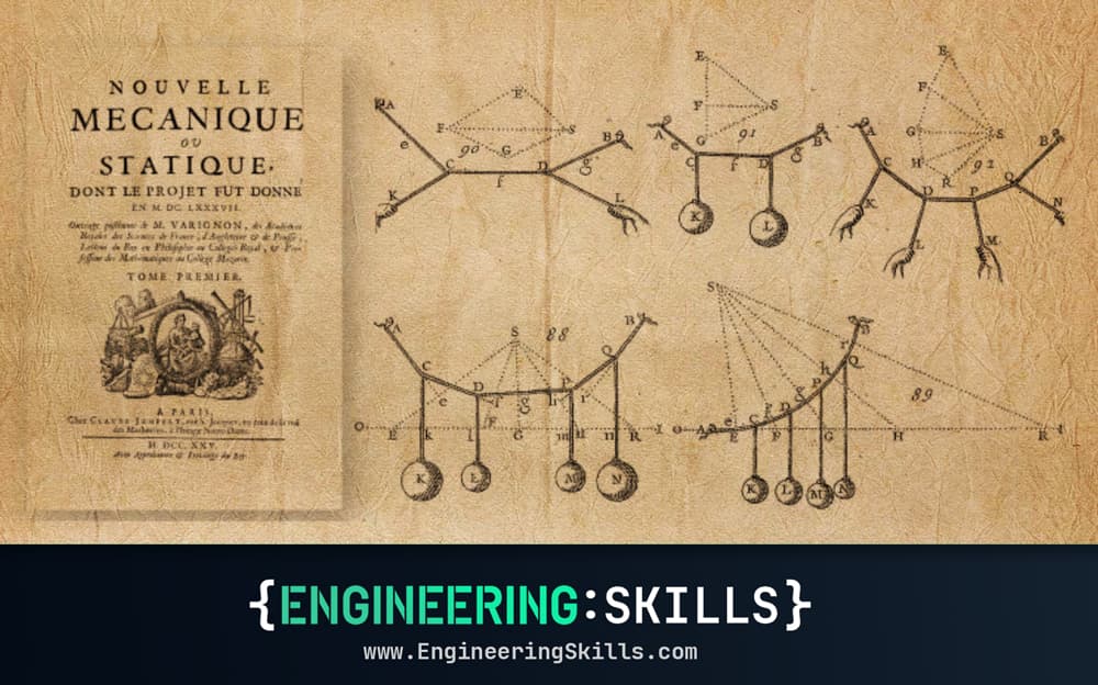
Getting Started with Graphic Statics
Rediscover the link between geometry and load flow with graphical structural analysis techniques.

Prof Edmond Saliklis