How to Calculate Beam Deflection
![[object Object]](/_next/image?url=%2Fimages%2Fauthors%2Fsean_carroll.png&w=256&q=75)
In this tutorial, you’ll learn how to calculate beam deflection from first principles using the differential equation of the deflection curve. We’ll cover several calculation techniques, including one called Macauley’s Method which greatly speeds up the calculation process. We’ll work our way through a couple of numerical examples before discussing how we can use the principle of superposition and tabulated formulae to speed up the process even further.
The table of contents below will give you an idea of what we’ll cover, but this tutorial is basically split into 3 chunks:
- Calculating beam deflection by integrating the differential equation of the deflection curve
- Speeding this process up with a clever technique called Macauley’s method
- The most practical (and fastest) approach which uses tabulated formulae and superposition
There is a lot in this tutorial, so give yourself plenty of time to work your way through it. Once complete, you’ll know pretty much all you need to calculate beam deflection and deflected shapes.
There is a lot in this tutorial, so give yourself plenty of time to work your way through it. Once complete, you’ll know pretty much all you need to calculate beam deflection and deflected shapes.
If you’ve landed on this post and are just after a table of beam deflection formulae, check out the table at the bottom of the page.
1.0 Differential Equation of the Deflection Curve
The differential equation of the deflection curve is used to describe bending behaviour so it crops up when examining beam bending and column buckling behaviour. The equation simply describes the shape of the deflection curve of a structural member undergoing bending. So, if measures the distance along a beam and represents the deflection of the beam, the equation says,
where, is the flexural rigidity of the beam and describes the bending moment in the beam as a function of . We won’t go into the derivation of the equation in this tutorial, rather we’ll focus on its application.
Our objective is to use this equation to calculate beam deflection, , so we need to integrate the equation twice to get an expression for . The best way to get to grips with this is to work through an example.
1.1 The ‘Small Deflection’ Assumption
Before we work our way through the example below we need to state the assumptions on which our analysis is based. The first is the so-called ‘small deflection’ assumption. In order to obtain equation 1, we made the assumption that the deflection of our beam (or any deflecting structure we apply this equation to) is small. In other words, if we consider a short curved length of our beam undergoing deflection, the curved length, , should be approximately equal to its length projection onto a horizontal plane, .
We also must assume that at any point along our beam, the rotation of the beam, is small enough that we can say , i.e. the angle of rotation at a point is approximately equal to the slope of the deflection curve. For most practical cases, deflection is a serviceability issue and we expect it to be relatively small and largely imperceptible to the naked eye. As such, this small deflection assumption is satisfied in most cases, but you need to be aware of its existence.
1.2 The Linearly Elastic Assumption
In order to derive equation 1 it was also assumed that the material the beam was made of was linearly elastic and therefore followed Hooke’s law. This must be the case because we are relying on the fact that the curvature of the beam, is proportional to the associated bending moment. This is important to remember, because our deflection equations will become inaccurate for plastic deformations, which would likely also invalidate our small deflection assumption. Now that we know the boundaries we’re working within, we can crack on with the example.
2.0 Determining the Bending Moment Equations
Consider the simply supported beam in Fig. 1 below. The beam is subject to two point loads and a uniformly distributed load. Our task is to determine the mid-span deflection and the maximum deflection. Note that because the beam isn’t symmetrically loaded, the maximum deflection need not occur at the mid-span location. Static analysis of the beam reveals the support reactions at and ,

Fig. 1. Simply supported beam.
Looking again at the differential equation of the deflection curve, we see that we need expressions that describe the bending moment as a function of . Looking at the loading here, we note that the bending moment diagram will not be described by one continuous function. The presence of two point loads means we’ll actually need three equations to fully describe how the bending moment varies along the beam; so, we’ll consider the beam as three different regions:
- Region 1:
- Region 2:
- Region 3:
where is measured from left to right with the origin at position . The equations for are obtained by making cuts in the structure to reveal the internal bending moment and then evaluating the internal bending moment as a function of by considering moment equilibrium of the sub-structure. If you’re unsure about any of that, take a detour over to this article on shear and moment diagrams for a refresher.
2.1 Internal Bending Moment in Region 1
To evaluate the internal bending moment in region 1, we cut the structure in this region to reveal the bending moment . Our cut is made at a distance to the right of support , Fig. 2.

Fig 2. Sub-structure created by the imaginary cut made in region 1. The cut reveals the internal bending moment in this region, .
Now, we know the sub-structure is in equilibrium under the action of the internal shear (not shown) and the internal bending moment. So we can evaluate moment equilibrium in order to determine an expression for .
Remember that this equation is valid for values for .
2.2 Internal Bending Moment in Region 2
We can repeat the process now to determine the relevant equation for region 2. Fig. 3. shows the sub-structure created by the cut to reveal the internal bending moment.

Fig 3. Sub-structure created by the imaginary cut made in region 2. The cut reveals the internal bending moment in this region, .
Evaluating the sum of the moments about the cut as above,
Again we note that this equation is valid for .
2.3 Internal Bending Moment in Region 3
Finally, we can establish the relevant equation for region 3, Fig. 4 below.

Fig 4. Sub-structure created by the imaginary cut made in region 3. The cut reveals the internal bending moment in this region, .
. Evaluating moment equilibrium of the sub-structure yields,
And again, for completeness we’ll note that this equation is valid only for .
3.0 Integrating the Differential Equation of the Deflection Curve
Now that we have established how the bending moment varies, we can substitute our relevant expressions for into the differential equation and perform our integrations. After substituting our expressions for into equation 1 we have,
Integrating each expression yields,
Here we note that our integration has generated three unknown constants of integration, , and . We also note that we now have the term in our equations which corresponds to the slope of the deflection curve. We need to perform one further integration to reduce this back to the displacement itself, . This integration yields,
Again we can see that this integration has given us a further 3 constants of integration, , and . In total we have six unknown constants that we need to identify. The good news is that we now finally have an equation for the deflection in each region.
3.1 Finding the constants of integration
In order to find the constants of integration, we need some conditions or constraints that we can represent in equation form. As we have six unknowns to solve for, we’re going to need 6 constraint equations. These are as follows:
- at , the slopes , in regions 1 and 2 are the same.
- at , the deflections , in regions 1 and 2 are the same.
- at , the slopes , in regions 2 and 3 are the same.
- at , the deflections , in regions 2 and 3 are the same.
- at (support A), the deflection is zero.
- at (support D), the deflection is zero.
The first four conditions are referred to as continuity conditions and result directly from the fact that the beam and therefore deflections and slopes are continuous. The final two are classic boundary conditions. We can now use these statements to build six equations from which the constants of integration can be identified.
Condition (1)
At , the slopes , in regions 1 and 2 are the same. Therefore we can equate equations 8 and 9 and substitute in .
Condition (2)
At , the deflections , in regions 1 and 2 are the same. So, equating equations 11 and 12 with gives us,
Condition (3)
At , the slopes , in regions 2 and 3 are the same, so using equations 9 and 10 with ,
Condition (4)
At , the deflections , in regions 2 and 3 are the same. Equating equations 12 and 13 with ,
Condition (5)
The fifth condition is a standard boundary condition; at the deflection is zero. So we can let equation 11 equal zero with ,
Condition (6)
The final condition relates to the other boundary; at the deflection is also zero. So applying this to equation 13 with gives,
Now that we have our six equations, we need to use them to solve for the unknown constants. By far the easiest way to do this is to arrange them in matrix form and solve the system by inverting the matrix of coefficients. The matrix representation of the system is,
The vector of unknown constants are obtained as,
At this point we need a way to invert a matrix, and as it’s a matrix, we won’t be doing this by hand! I’ll use the following Python code to perform the operation in equation 21.
import numpy as np #Numpy for working with arrays

#Define each row of the coefficient matrix
row1 = [1, -1, 0, 0, 0, 0]
row2 = [3, -3, 0, 1, -1, 0]
row3 = [0, 1, -1, 0, 0, 0,]
row4 = [0, 6, -6, 0, 1, -1]
row5 = [0, 0, 0, 1, 0, 0]
row6 = [0, 0, 8, 0, 0, 1]

A = np.mat([row1,row2,row3,row4,row5,row6]) #Define matrix of coefficients
B = np.array([[337.5],[675],[900],[3600],[0],[-14613.334]])

C = A.I*B #Unknown constants
If you want to get Python set up on your machine, you can follow this lecture. This will get you set up with a handy Python coding environment. Assuming you’ve done that, or have your own way of inverting matrices, the constants evaluate to,
4.0 Calculating Beam Deflection
At this point we can summarise the three equations that describe the deflection in the three regions of our beam:
4.1 Mid-span beam deflection
To calculate the mid-span beam deflection, we substitute into equation 23 giving us,
Now that we have a complete definition of the deflection in the beam, we can plot it to get a better sense of the deflected shape. Fig. 5 below shows a plot of the internal bending moment and the deflected shape. Note the y-axis gives the deflection is a function of .
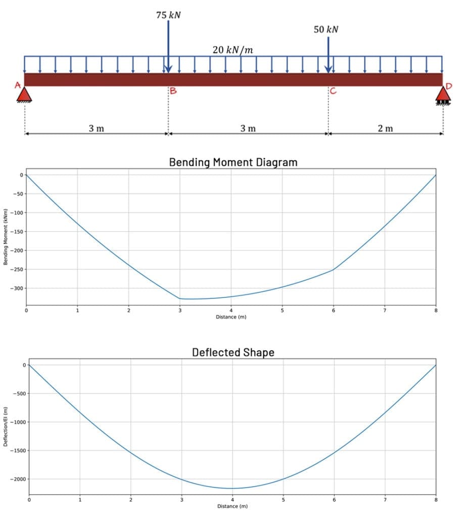
Fig. 5. Simply supported beam, plot of bending moment and plot of deflected shape.
4.2 Location of Maximum Beam Deflection
We can see from Fig. 5 above that despite the unsymmetrical loading, the maximum deflection occurs very close to the mid-span location. We can confirm the exact location of the maximum deflection by recognising that at this location, the slope of the deflection curve is zero. In other words, a tangent to the deflection curve at the point of max deflection would be horizontal and therefore have a slope of zero.
We know by inspection that the max deflection occurs in region 2. But let’s assume we didn’t know this. We can let each equation for the slope of the deflection curve, , equations 8, 9 and 10, equal to zero and solve for the roots of each equation, i.e. the values of x at which the slope is zero. I’m going to let Python do the manual labour here…
#Define the polynomials
p1 = np.poly1d([-10/3, 139.375/2, 0, -856.354]) #Region 1
p2 = np.poly1d([-10/3, 64.375/2, 225, -1193.854]) #Region 2
p3 = np.poly1d([-10/3, 14.375/2, 525, -2093.854]) #Region 3

#Extract the roots
rootRegion1 = p1.r #Region 1
rootRegion2 = p2.r #Region 2
rootRegion3 = p3.r #Region 3
The roots are,
Values that fall outside the boundaries of the relevant region can be immediately discarded. This leaves only in region 2. As we suspected, this is very close to the mid-span location. We could now substitute this value back into equation 12 to confirm the value of max deflection but since we’ve already worked out the deflection at , we won’t bother doing this.
5.0 Speeding up beam deflection calculations with Macauley’s method
You’ll probably agree that the calculation process up to this point has been quite laborious. We can speed the whole process up considerably using a technique called Macauley’s method. It’s also known as the singularity function method and we’ll cover this next.
We’ve seen that the basic process of calculating beam deflection involves evaluating an expression for the bending moment as a function of , the coordinate along the beam. We can substitute this expression into the differential equation of the deflection curve and perform a double integration to produce a closed-form solution (an equation) for the deflection as a function of .
Now, since our bending moment diagram was not a continuous function of , we needed to break up our bending moment diagram into segments where a single continuous function defined each segment. The double integration required for each segment yielded two unknown constants of integration. This was all perfectly solvable, but the process is generally very tedious for anything other than very simple loading.
5.1 How does Macauley’s Method help?
This is where Macauley’s method comes in. I’ll outline the headlines here – but this is only really going to make sense when we work through an example in the next section – so don’t worry if the following leaves you scratching your head! Macauley’s method is really just an alternative method or process we can use to evaluate the differential equation of the deflection curve. The method works by introducing a singularity function (hence the alternative name), which allows us to discount or ignore certain terms in the bending moment function .
So, instead of building three different functions for the bending moment in the question above, we would build a single equation for by cutting the beam between C and D, thereby capturing the moment influence of all loads on the structure. The ‘trick’ that Macauley’s method introduces is that we multiply each term in the bending moment equation by a singularity function (will make more sense below) that we let equal to zero when it has a value less than one. The way we implement this allows us to cleverly eliminate terms from the moment equation when we’re evaluating sections of the beam, where those terms are not relevant.
For example, if we cut the beam above between B and C and consider equilibrium of the sub-structure to the left of the cut, the point load would feature in the moment equation but the would not. Macauley’s method simply allows us to construct a single moment equation and eliminate any non-relevant terms. This method results in us performing double integration on one equation (not three) yielding only two unknown constants of integration – greatly reducing our workload. In the next section we’ll flesh out this idea with an example.
6.0 Beam Deflection – Macauley’s Method Example
To demonstrate the benefits of Macauley’s method, let’s start by re-analysing the beam. We’ll break the process up into discrete repeatable steps that you can replicate on other beams.
6.1 Step 1: Sub-structure setup
We need to generate an equation that describes the internal bending moment as a function of . To do this, we make a cut in the structure at some distance to the right of the left support. We’ll treat the left-most tip of the beam as the origin of our x-axis.
When implementing Macauley’s method, we make sure we cut the structure at a location that allows us to consider all of the actions (applied forces and moments) to the left of the cut. This typically means making a cut some infinitesimally small distance to the left of the right tip of the beam. When taking moments about the cut, notice that all of our lever arm terms contain . This is critical as these lever arm terms will be treated as our singularity functions.
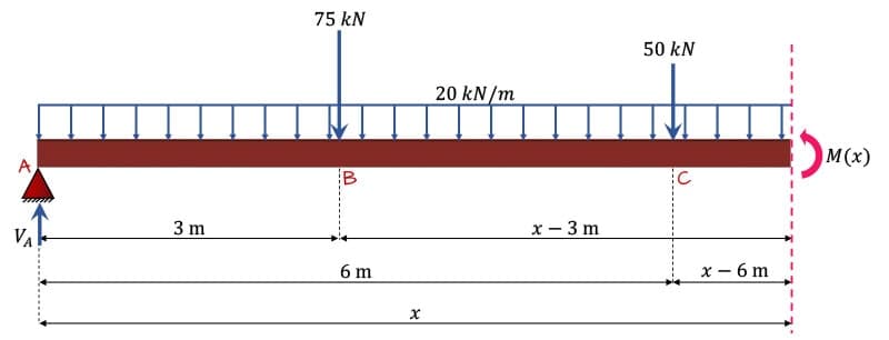
Fig. 6: Sub-structure for Macauley’s method analysis
6.2 Step 2: Build an expression for with singularity functions
Taking moments about the cut and recalling the vertical reaction at A was previously determined to be , yields the following expression for ,
**Pay special attention to the terms in square brackets, these are our singularity functions. Macauley’s method says that when the terms in brackets evaluate to a negative number, we treat the term in brackets as a zero.**Think about this for a minute – what is this actually saying? Imagine we make a cut in the structure at to determine the internal bending moment at this location by considering equilibrium of the sub-structure to the left of the cut. Naturally the force at C would not feature in this equation. The ‘rule’ we just implemented caters for this since the singularity function for the force would evaluate to and according to Macauley’s method, this would be eliminated from the equation! Therefore after applying Macauley’s method to the moment expression we would have,
You can think of what we’ve done so far as building the most complete expression for the internal bending moment and then implementing a rule that allows us to eliminate terms from the expression as required.
6.3 Step 3: Integrate the differential equation of the deflection curve
Now we can substitute our expression for the internal bending moment, complete with singularity functions (which are really just the lever arm expressions) into the differential equation of the deflection curve and integrate the equation.
Before integrating, note that we are keeping the singularity functions intact and not expanding them or multiplying through the terms to the left of the brackets. After integrating twice we end up with,
where and are the constants of integration.
6.4 Step 4: Apply boundary conditions and solve for constants of integration
We can now apply our boundary conditions in the usual way to determine the unknown constants and .
Boundary condition 1:
At the deflection . Note that when , all of our singularity functions either become zero or negative which according to Macauley’s method we treat as zero,
Therefore, .
Boundary condition 2:
At , . This boundary condition yields,
Since , we end up with . Therefore our final equation for the deflection becomes,
This essentially marks the end of the process and we can now use our equation to evaluate the deflection as required. So for example, let’s consider the deflection at the mid-span location, at . Substituting into our equation and observing Macauley’s method of eliminating terms where the singularity function evaluates to a negative would yield,
We can confirm that this is the same value we derived in our first analysis. However, we only needed to integrate a single equation and evaluate two unknown constants of integration. The process was a lot quicker this time around. In a nutshell, this is Macauley’s method – fundamentally we’re still integrating the differential equation of the deflection curve, we’re just being a little smarter about it.
7.0 Plotting the deflected shape
Once we have our equation for the deflection, an excellent next step would be plotting the equation and visualising the deflected shape of the beam. We can write a simple algorithm to achieve this. I’ll use Python inside a Jupyter notebook, but you can use any language you’re comfortable with. If you’re new to Python, take a look at this project that will help you get up and running with little or no experience.
The first thing I do inside a blank Jupyter notebook is import some packages to give me additional functionality. On line 2 below, I import Numpy to help me work with arrays of numbers, and on lines 3-5, I’m importing Plotly, a graphing library that helps me produce nice graphs.
import numpy as np #Numpy for working with arrays
import plotly as py #Import Plotly
import plotly.graph_objs as go #Import graph objects
py.offline.init_notebook_mode(connected=True) #Setup offline plotting (inside Jupyter notebook)
With these preliminaries out of the way, we can get on to the core of the code. In lines 3-6 below we set up a range of x-coordinates along the length of the beam. On line 10 we initialise a container to hold the value of deflection at each x-coordinate and on line 11 we establish a for loop to cycle through each x-coordinate and calculate the value of deflection at each point.
We’ve divided the expression for deflection into different parts which allows us to use if conditions to test if the current value of renders the singularity function zero or not. This way we’re implementing Macauley’s method and only taking into account the relevant parts of the deflection equation for each position on the beam.
After stepping through all of our test conditions and building up our deflection for the current location, we save that value on line 39 and move onto the next x-location with the next iteration of our for loop and repeat the process all over again.
#Defaults and initialisations
span = 8
divs = 10000 #Divide span up into this number data points
delta = span/divs #Distance between data points
X = np.arange(0,span + delta,delta) #Range of x-coordinates
EI = 1

#Cycle through the structure and calculate the deflection at each point
Deflection = np.zeros(len(X)) #Initialise a container to hold all deflections
for i, x in enumerate(X):
  deflection = 0

  #Term 1, 3 and 5
  if x > 0:
    #Reaction
    delta = (139.375/6)*x**3
    deflection = deflection + delta

    #UDL
    delta = -(20/24)*x**4
    deflection = deflection + delta

    #C1
    delta = -856.4*x
    deflection = deflection + delta

  #Term 2 - 75kN point load
  if x-3 > 0:
    delta = -(75/6)*(x-3)**3
    deflection = deflection + delta

  #Term 4 - 50 kN point load
  if x-6 > 0:
    delta = -(50/6)*(x-6)**3
    deflection = deflection + delta

  #Store deflection for this location
  Deflection[i] = deflection/EI
Now that we’ve calculated an array of deflection values for each position along the beam, we can use Plotly to visualise them. The code below is pretty standard plotting code for Plotly. You can use whatever programme or library you like to visualise the deflection; all you’re doing is plotting a range of x versus y values. I include the code below more for completeness than anything else.
#Define a layout object
layout = go.Layout(
  title={'text': "Deflection"},
  yaxis = dict(title='Deflection/EI (m)'),
  xaxis = dict(title='Distance (m)'),
  showlegend=False
)

#Define the deflection line
line = go.Scatter(
  x = X,
  y = Deflection,
  mode='lines',
  name='Deflection'
)

#Define a horizontal line to represent the structure
axis = go.Scatter(
  x = [0, span],
  y = [0,0],
  mode='lines',
  line_color='black'
)

#Generate and view the figure
fig = go.Figure(data=[line, axis], layout=layout)
py.offline.iplot(fig)
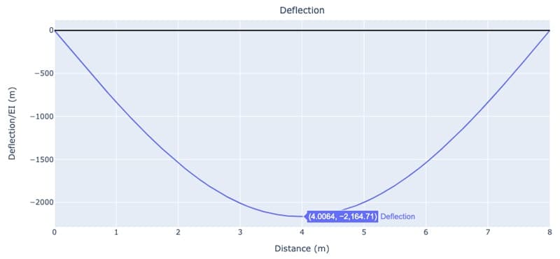
Fig. 7: Beam deflection obtained using Macauley’s method.
Although I’ve used two different plotting libraries to plot the deflection from each analysis, we can still compare figures 5 and 7 to confirm that we’ve achieved the same result.
8.0 A Tougher Beam Deflection Example – Macauley’s Method with Partial UDLs and Point Moments
The previous example demonstrated the advantages of Macauley’s method over our previous approach to calculating the deflection. However, before we wrap up our discussion, we should probably work through a slightly more challenging example question. This will give us the chance to address partial uniformly distributed loads (patch loads) and point moments.
To use Macauley’s method to deal with these actions, we need to implement specific strategies. So with this in mind, consider the structure below. Our task is to plot the deflected shape for the structure as we did for the previous example. We’ll also determine the magnitude and location of the maximum deflection between A and B.

Fig. 8: Example beam.
8.1 Beam reactions
We can start by calculating the vertical reactions at A and B. Taking the sum of the moments about point A,
Evaluating the sum of the forces in the vertical direction yields .
8.2 Macauley’s method and patch loading
The arrangement of loads on our structure causes us two problems that we’ll need to consider if we’re to use Macauley’s method,
- the fact that the distributed load doesn’t run all the way to the end of the beam on the right hand side causes us a problem which we’ll solve next.
- the existence of a moment needs to be addressed – because this does not have a lever arm, we don’t naturally have a singularity function that we can apply to it – this one is an easy fix which we’ll see shortly.
Let’s simplify things for demonstration purposes and imagine our beam only had a distributed load acting on it. We can set up the sub-structure to the left of the cut as shown below in Fig. 9.
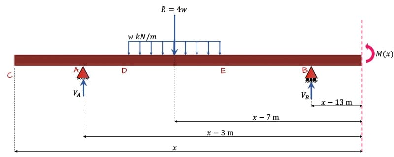
Fig. 9: Sub-structure with uniformly distributed load only.
Our expression for the bending moment at the cut would be,
Notice that our expression has the full UDL, ‘baked’ into it. This means that this equation can only be valid for values of . This typically wouldn’t be a problem because our singularity functions usually eliminate the influence of a load when the cut is to the left of the load. However, notice that the singularity function only eliminates the influence of the UDL when . So there is a window when $7 To overcome this we need our UDL to always run to the end of the beam, in other words our vertical cut must always cut through whatever UDLs are applied to the beam. An easy way to satisfy this requirement is to extend our UDL to the end of the beam and then apply a UDL in the opposite direction to cancel the influence of the extra UDL we’ve added – this makes more sense when you see it in action, Fig. 10 below.
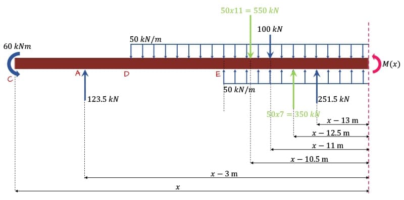
Fig. 10: Sub-structure with all example loading shown. Note that the forces in green are the resultants of the UDL loads.
The combined influence of both UDLs in Fig. 10 is the same as the influence of the single UDL shown in Fig. 8.
8.3 Macauley’s method and point moments
We said above that the existence of point moments caused a problem because a moment doesn’t get multiplied by a lever arm in our moment equation and therefore there is no singularity function to eliminate the moment when it doesn’t contribute to . Now in our example question this problem never actually arises because the moment at C will always feature in the equation for , i.e. we never evaluate the internal bending moment to the left of the , because it’s applied at the end of the beam.
However, to illustrate the problem and solution for future reference, let’s imagine the same beam with a moment, applied at say , Fig. 11 below. In this case the internal moment expression would be,

Fig. 11: Sub-structure with single point moment applied.
Currently we have no way of eliminating the moment when . However if we introduce a ‘sudo’ lever arm, , we give ourselves a singularity function that enables us to apply Macauley’s method to this moment and eliminate it. Note that , so we never actually alter the magnitude of the moment when it should feature in our equation. So, the complete expression for the internal moment, that we can apply Macauley’s method to is,
But as we said, we don’t need to implement this ‘fix’ in our example because the moment will always feature in our equation because it’s positioned on the extreme left end of the beam. So, with these two details covered, we can get back to solving our question.
8.4 Build an expression for with singularity functions and integrate
We have the complete sub-structure with all loading and lever arms shown in Fig. 10 above. Taking moments about the cut we can build our expression for as follows,
We now substitute this expression into our differential equation of the deflection curve,
Integrating to obtain an expression for the slope,
Integrating again to obtain our expression for the displacement,
Boundary condition 1: :
Applying the boundary condition for the displacement at A yields,
Boundary condition 2: :
The boundary condition for the displacement at B yields,
Solving the simultaneous boundary condition equations we obtain and . Therefore our final expression for the displacement of the beam is obtained as,
8.5 Plotting the deflected shape
We will employ the exact same technique as before to plot the deflected shape. The code below is structured the same as the code we’ve seen above, but the contents are obviously altered to represent our new deflection equation. The code to produce the plot is the same and is not repeated below.
#Defaults and initialisations
span = 16
divs = 10000 #Divide span up into this number data points
delta = span/divs #Distance between data points
X = np.arange(0,span + delta,delta) #Range of x-coordinates
EI = 1

#Cycle through the structure and calculate the deflection at each point
Deflection = np.zeros(len(X)) #Initialise a container to hold all deflections

for i, x in enumerate(X):
  deflection = 0

  #Term 1 and 7
  if x > 0:
    #Moment
    delta = -(60/2)*x**2
    deflection = deflection + delta

    #C1
    delta = -765*x
    deflection = deflection + delta

  #Term 2 - Reaction at A
  if x-3 > 0:
    delta = (123.5/6)*(x-3)**3
    deflection = deflection + delta

  #Term 3 - 50 kN/m UDL acting downwards
  if x-5 > 0:
    delta = -(50/24)*(x-5)**4
    deflection = deflection + delta

  #Term 4 - 100kN point load
  if x-11 > 0:
    delta = -(100/6)*(x-11)**3
    deflection = deflection + delta

  #Term 5 - 50 kN/m UDL acting upwards
  if x-9 > 0:
    delta = (50/24)*(x-9)**4
    deflection = deflection + delta

  #Term 6 - Reaction at B
  if x-13 > 0:
    delta = (251.5/6)*(x-13)**3
    deflection = deflection + delta

  #Term 7 - C2
  deflection = deflection + 2565

  #Store deflection for this location
  Deflection[i] = deflection/EI
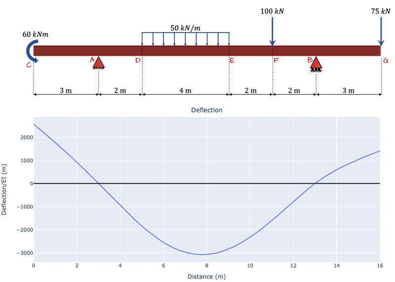
Fig. 12. Deflected shape for the beam. Note that in the calculation, the flexural rigidity EI is assumed to be 1 for convenience.
It might seem odd that the point load at G is never directly featured in our internal bending moment equation, . However, its influence is taken into account indirectly through the reactions at A and B. You can confirm this by simply increasing the point load to say and repeating the calculation. This will require you to calculate new reactions, re-evaluate the constants of integration and slightly amend the code block above to capture the changes – but it’s not as laborious as it sounds. I’ve plotted a comparison of the two deflections in Fig. 13 below.
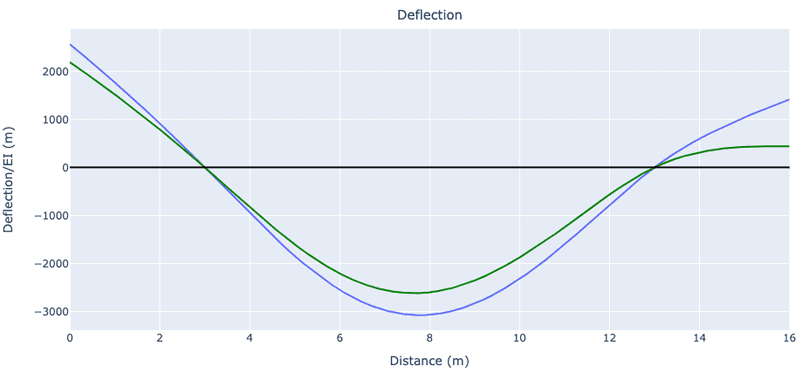
Fig. 13: Comparison of deflected shapes for a 75 kN point load at G (blue) and a 100 kN point load at G (green)
The influence of the larger point load at G is clearly visible and qualitatively it’s exactly what we would expect.
8.6 Maximum deflection between A and B
The last thing we want to tackle is identifying the location and magnitude of the maximum span deflection between A and B. This is relatively easy to obtain as the maximum deflection occurs where the slope of the deflected shape is zero. Fortunately, we have an equation for the slope already – so we just need to let it equal to zero and solve for x…easier said than done! Take a look at the equation again (repeated from above),
Solving this equation algebraically for is too difficult. A much more practical approach is to identify the region of interest visually, say between meters and use trial and error, i.e. plug values of into the equation and see which one makes the equation equal to zero. In the dark ages, one might have done this by hand – but lucky for us we can put a robot on the job instead – via a Python script!
Our approach will be to use a for loop to cycle along each position on the beam and calculate the slope in much the same way that we calculated the deflection. At the end of each loop iteration, we’ll test if the sign of the slope has changed from negative to positive. When it has, it means that the point of zero slope was crossed between the previous and current iteration. We’ll take the x-position on the current iteration as the point at which the slope was zero and, therefore, the location of the maximum deflection.
previousSlope = 0 #Slope from previous iteration (initialise a value)
for i, x in enumerate(X):
  slope = 0 #Slope calculated on this iteration

  #Term 1 - Moment
  if x>0:
    delta = -60*x
    slope = slope + delta

    #Term 2 - Reaction at A
    if x-3 > 0:
      delta = (123.5/2)*(x-3)**2
      slope = slope + delta

    #Term 3 - 50 kN/m UDL acting down
    if x-5 > 0:
      delta = -(50/6)*(x-5)**3
      slope = slope + delta

    #Term 4 - 100kN point load
    if x-11 > 0:
      delta = -(100/2)_(x-11)**2
      slope = slope + delta

    #Term 5 - 50 kN/m UDL acting up
    if x-9 > 0:
      delta = (50/6)_(x-9)**3
      slope = slope + delta

    #Term 6 - Reaction at B
    if x-13 > 0:
      delta = (251.5/2)*(x-13)**2
      slope = slope + delta

    #Term 7 - C1
    slope = slope - 765

    #Test for change in sign if slope
    if i>0 and x>7.5 and x < 10:
      if previousSlope<=0 and slope>0:
        location = x

    previousSlope = slope #Update the value of previousSlope for the next iteration

#Print a statement to show the end result
print('The maximum deflection between A and B occurs at x={one} m'.format(one=round(location,3)))
Our script outputs the following text string,
The maximum deflection between A and B occurs at x=7.781 m
We can now substitute this value for in our deflection equation and obtain the deflection at this location,
That wraps up our Macauley’s Method analysis. In the days of computerised structural analysis, we rarely need to process a deflection like this – but it’s still nice to keep in touch with the fundamental principles. Next, we’ll look at some even quicker ways of determining beam deflection that avoid calculus completely.
9.0 Using Superposition to Calculate Beam Deflection
We’ve seen above how to determine beam deflection from first principles. It has given us a complete picture of the deflection, but even after employing Macauley’s Method, it’s still been a relatively lengthy process to calculate a deflected shape.
We can make use of the principle of superposition to arrive at an answer for the mid-span deflection much faster by making use of tabulated formulae for beam deflection. These formulae have already been determined and tabulated for common load cases using the technique we’ve just demonstrated. Some of the more common deflection equations are summaries in the table below.
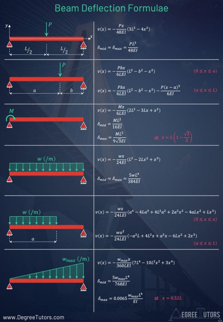
Fig 14. Beam deflection table with some common beam loading arrangements.
Relying on the principle of superposition, we can evaluate the mid-span deflection for each load individually and then simply add or superimpose the deflections together. Doing so will yield the same result identified above.
9.1 Uniformly Distributed Load
Consider the formula for the deflection of the beam subject to a uniformly distributed load, Fig. 15,
At , this formula evaluates to .

Fig. 15. Simply supported beam subject to a uniformly distributed load.
9.2 Point Load #1
The formula for the deflection of a beam subject to a single point load, Fig. 16, where the distance is less than the distance to the position at which the deflection is being evaluated, is,
This evaluates to
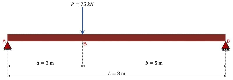
Fig. 16. Simply supported beam subject to a point load at a distance from the left support and from the right support.
9.3 Point Load #2
Finally, evaluating the formula for deflection where , Fig. 17,
This evaluates to .
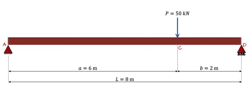
Fig. 17. Simply supported beam subject to a point load at a distance from the left support and from the right support.
Summing up the three mid-span deflections yields,
Sure enough, this is the same value we obtained above. By plotting these equations, we can further visualise the contribution of each load towards the overall deflected shape, Fig. 18.
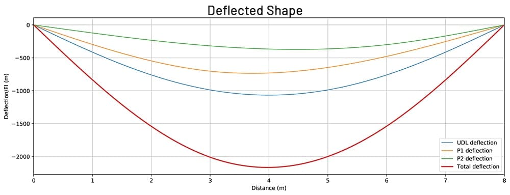
Fig. 18. Total deflected shape obtained as the superposition of individual deflections from each load considered separately.
So that about wraps up our discussion of beam deflection. In the end, it’s up to you what approach you decide to take to calculate deflections. There are of course other methods that you may use to evaluate deflection, but in any event it’s good to have an understanding of how we can go about it from first principles. Remember, just like any derivation, this one has its limiting assumptions, discussed above. Everything we’ve discussed above is only valid provided we satisfy these limiting assumptions.
If you found this post helpful, you might like this project where we build a beam deflection calculator in Python – if you think Macauley’s Method is fast, building your own calculator makes calculating beam deflections lightning fast.
That’s all for now, I’ll see you in the next one.
Dr Seán Carroll's latest courses.



Featured Tutorials and Guides
If you found this tutorial helpful, you might enjoy some of these other tutorials.
A practical guide to floor vibration serviceability assessment
Part 1: Understanding human-induced floor vibration and assessing acceptability

Dr Seán Carroll
