3D Truss Calculator – Quick Start Guide

Welcome to this quick start guide on how to use the 3D truss calculator. To get up and running as quickly as possible, read through this tutorial or watch the video walkthrough below. If you’ve already used the 2D truss analysis toolbox, the good news is that the 3D version works exactly the same way. If you’re completely new to both, by the end of this tutorial, you should be comfortable analysing your own structures. We’ll work through the solution of a sample structure, the data for which can be accessed by clicking the Example Data button below the 3D viewport (on the solver page).

🧰 Go to the Free 3D Truss Calculator

If you’re more interested in how to perform the underlying structural calculations, then take a look at this course on 3D Space Frame analysis. This online toolbox is based on the truss analysis calculator we build in that course.

🛠 We also have a free 2D truss calculator for simpler structures – check that out here.

If you’re just learning about truss analysis using the method of sections or the method of joints, go here first – it’s a great way to generate example questions for yourself to solve and improve your manual analysis skills.

Step 1 – Defining the structure

The structure we’re going to model is a lattice tower, based on the type of structure you might find supporting power lines. It’s suitable for this analysis because it’s essentially a 3D truss – all members are assumed to be axially loaded. This solver only deals with structures that consist of axially loaded members – no bending or shear (yet!).

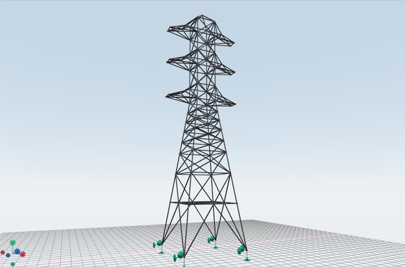
Fig 1. 3D truss or ‘space frame’ structure to be analysed.

As mentioned above, the data for this structure has already been generated and is freely accessible so you can follow along with this tutorial. But when you move beyond this tutorial, you’ll quickly find that generating the data for any sizable 3D structure becomes a huge bottleneck. It’s just really time-consuming to manually determine the coordinates of all nodes and then define the members that connect between these nodes.

So, I’ve created a Blender template modelling file with some custom scripts. You can use this file to model your structure and easily generate the nodal, element, restraint and force data for your structure. The data generated can be directly copied into the solver data entry boxes. You can access the template file by clicking the Modelling Template button beside the Example Data button on the solver page. I won’t cover it in this article, but you can watch the video tutorial above to see how the template file is used, Fig. 2.

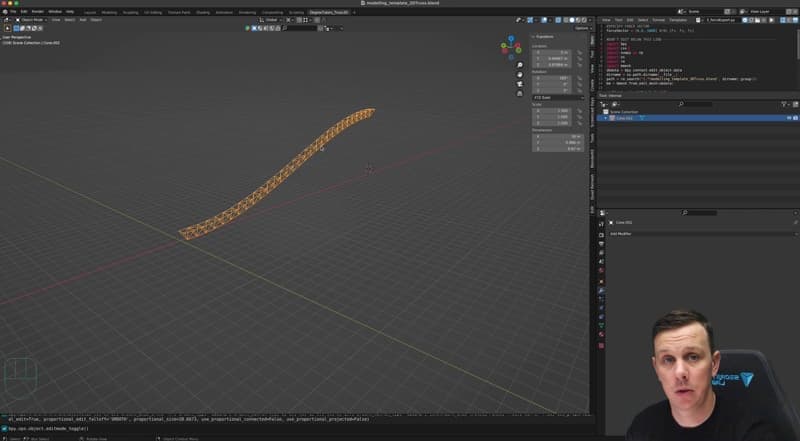
Fig 2a. The Blender modelling template can be used to generate structural models.

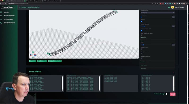
Fig 2b. The data exported from the modelling template can be used directly inside the truss analysis toolbox.

Nodes

We start by defining the positions of each node in the structure. This is done by specifying x, y and z coordinates. The nodal information can be copied and pasted directly from the table of sample data. Make sure to only copy the data contained within the green cells on the google sheet, Fig 3.

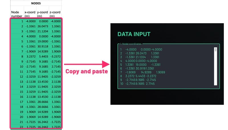
Fig 3. Copying node information from the sample data spreadsheet into the data entry box.

You can type data manually into the data entry boxes within the solver, but it’s usually much more convenient to collect your data in a spreadsheet and simply copy and paste it over to the solver. Note that the first column of numbers are sequential node numbers. Once the node information is pasted in, the nodes will appear in the 3D viewport, Fig 4.

Note that to generate the image in Fig. 4, I have changed the 3D viewport to a perspective projection (the default is orthographic) and increased the scale parameter to improve visibility. I have also disabled ‘Reset viewport on update’ to stop the viewpoint resetting as viewport options are changed. All of these options are accessed from the right-side control panel.

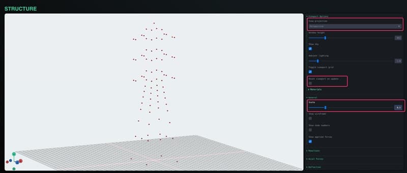
Fig 4. Nodes in the 3D viewport, note that perspective projection, viewport update and structure scale have been edited in the right side control panel.

Members/Elements

The element information is added next. Again, each element is defined on a new line with a complete definition consisting of:

• Member number
• Node number at end i (referencing the node numbers set in the previous data entry box)
• Node number at end j (referencing the node numbers set in the previous data entry box)
• Material (Young’s) modulus
• Cross-sectional area
• Yield stress
• Self-weight

Once the element data is pasted in, the 3D viewport updates accordingly, Fig 5.

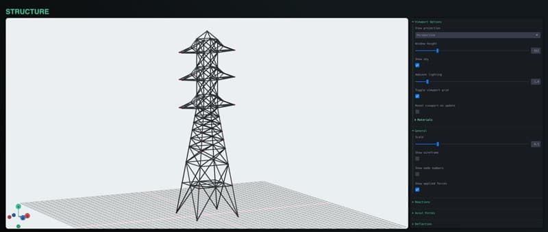
Fig 5. 3D viewport after element definitions have been added.

Step 2 – Defining supports/restraints

Restraint information is added to the third data entry box. To define a restraint, we simply specify a node number and type TRUE or FALSE to indicate restraint in the respective global x, y or z direction. Again, I recommend maintaining a record in a separate excel file and copying and pasting across. The 3D viewport will update with every complete restraint definition added, Fig. 6.

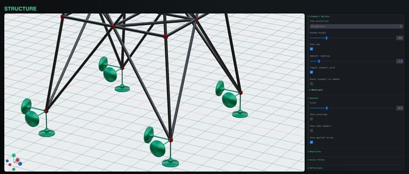
Fig 6. Full pin (x, y and z) restraints specified for nodes 1, 4, 51 and 52.

Step 3 – Defining applied forces

The applied forces are specified in much the same way as restraints in that we specify the relevant node number first, followed by the x, y and z components of force applied to that node. So, in this case, we’re applying a 5kN force in the negative y-direction to the nodes specified. The forces will appear in the 3D viewport as they’re added to the data entry box. The force visibility can be toggled on and off in the 3D viewport from the General section of the control panel to the right of the viewport.

In addition to specifying point loads on any node, we can also toggle self-weight on and off. This will optionally add the self-weight force to the structure so that the returned results will reflect the influence of self-weight.

Reviewing the 3D truss calculator results

Once all of the data has been entered, you can hit the SOLVE button to submit your analysis. Your results should be returned straight away, although there might be a short delay if there are a lot of requests being submitted simultaneously. When your job is complete, and results are returned, several different results tables will appear. You’ll also be able to review your results data in the 3D viewport. The best thing to do at this point is simply to poke around yourself and switch things on and off to get a better understanding of how the results are displayed. But I’ll briefly cover your options below. Note that once you submit your job, the data entry block will collapse – it hasn’t disappeared. You can bring it back (along with your entry data) by expanding the data entry panel.

Analysis report

The first thing to review is the analysis report summary, Fig 7. This gives a high-level overview of how your analysis went. You can read the details line by line, but the headline is you should see a full list of green tick marks. If there are any red error indicators, then something went wrong. If something goes wrong, you most likely won’t have results reported back. But if you do, you should disregard them and investigate what might have caused your analysis to fail. This may be something to do with how you defined your structure.

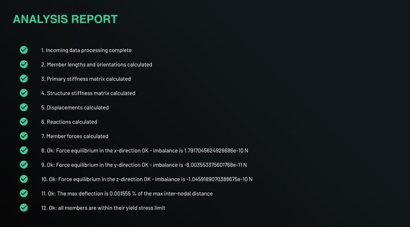
Fig 7. Analysis report.

Pay particular attention to items numbered 8 to 12. Checks 8, 9 and 10 evaluate force equilibrium in the x, y and z directions and report the difference between applied forces and reactions. This number should theoretically be zero, although it will typically be a very small number due to the way small numbers are handled within programming languages.

Check 11 calculates the maximum nodal deflection as a proportion of the largest inter-nodal distance in the structure. This gives an indication as to whether or not the calculated deflections are too large. Very large deflections, in comparison to the scale of the structure, suggest the structure and/or loading merit further investigation as geometric non-linearity may occur (we discuss this in detail in this course). The toolbox will issue a warning if the deflection exceeds 10% of the maximum inter-nodal distance, but this limit is itself arbitrary. You must use your own engineering judgement to assess the acceptability of deflections.

Check 12 indicates if any members have exceeded their specified yield stress. In order for the truss calculator results to be valid, all members must remain within their elastic range. Otherwise, material non-linearity will lead to the calculator results being inaccurate. This is one of the easiest things to overlook in a simple truss analysis, so watch out for a red warning sign here.

Table data

The reactions, axial forces and nodal displacements are presented in the three tables below the analysis report, Fig 8. If you’re a EngineeringSkills member and logged in, you can download the data from each table in csv file format. The table functionality is all fairly intuitive so I won’t labour each individual piece of functionality here.

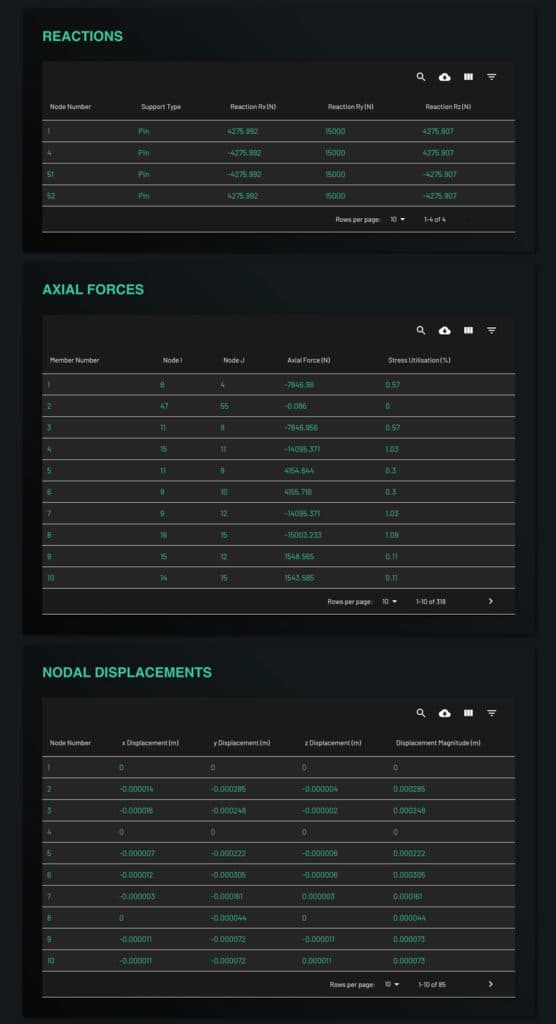
Fig 8. Reactions, axial forces and nodal displacements data tables.

Reviewing results in the 3D window

The best way to get a quick sense of how the structure responds to the applied loads is by reviewing results in the 3D window. For the best overview of the 3D window and its data visualisation functionality, you should watch the getting started video. Alternatively, just play around with the control panel on the right. You’ll get the hang of what each toggle and widget does pretty quickly, but I’ll briefly outline the functionality here.

Axial forces and reactions

The axial force view can be toggled on and off from the Axial Forces section of the control panel. The colour of the members indicates the magnitude of axial force and corresponds with the colour scale below the 3D viewport. You can view the members coloured by a continuous scale or a binary scale that simply indicates tension (blue) and compression (red). From the Axial Forces section of the control panel, you can also toggle force labels on or off.

The support reactions can be toggled on and off from the Reactions section of the control panel. Toggling the reactions on will replace the supports with reaction force arrows indicating the direction of the reaction forces. The magnitude is indicated with an annotation.

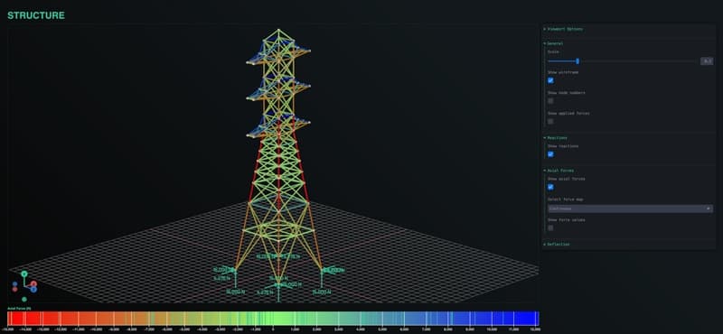
Fig 9. Axial forces and reactions in the 3D view.

Deflected Shape and Nodal Displacements

The deflected shape of the structure can be toggled on and off as well as annotations showing the nodal displacements in the x, y and z directions. Just like the axial force annotations, these labels can be quite dense when viewed across the whole structure. So, it’s best to zoom into an area of interest before toggling the labels on. The deflection can be scaled using the slider in the Deflection section of the control panel. This makes it easier to determine the qualitative deflected shape when the deflections are too small to be perceived against the scale of the structure.

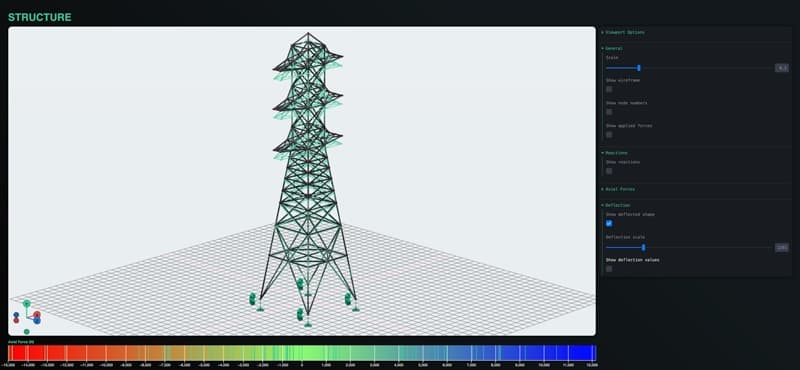
Fig 10. Deflected shape.

Wrapping up

That’s more or less all you need to know to get up and running with this 3D truss analysis toolbox. The rest of the options in the control panel are all self-explanatory, so as I said above, just play around with it, and you’ll get the hang of it. My hope is that students, in particular, will find this toolbox helpful for quickly generating analysis data for 3D pin-jointed structures as part of student design projects.

As you’ll see, if you watch the tutorial video at the top of this post, the toolbox becomes much more powerful when you team it up with Blender for creating your structural models. By modelling in Blender and using the exported data to feed the toolbox for analysis, you can quickly iterate on designs and explore how different configurations respond to loading. If you’re not already familiar with Blender, I can’t encourage you enough to give it a go – you’ll be amazed just how easy it is to develop complex 3D structural models using only a handful of commands.

That’s all for now. I hope you find this truss analysis toolbox useful – if you do, tell someone else who might also find it helpful.