Building a Mohr’s Circle Calculator for Stress Analysis in Python
![[object Object]](/_next/image?url=%2Fimages%2Fauthors%2Fsean_carroll.png&w=256&q=75)
1. How we’re going build a Mohr’s Circle Calculator using Python
In this Python project we’re going to build a Mohr’s Circle calculator. By the end of this project, you will have built your own stress analysis Python code. You’ll also have enough knowledge to expand and personalise your code to your own needs. Along the way we’ll cover all of the fundamental topics that lead up to Mohr’s circle of stress. You will learn about:
- how we use the 2D stress element to represent the state of stress at a point
- the purpose of stress transformation equations
- principal stresses and principal planes
- planes of maximum shear stress
- and of course Mohr’s circle!
You don’t need to be a Python programmer to work through this project!
We’ll be using the Jupyter Notebook development environment to write our Python code. If you’re new to Jupyter Notebooks (or Python) and need a little help getting up and running – check out this lecture (part of another course but covers what you need to get up and running).
If you’re new to Python, don’t let it intimidate you! Once you get comfortable with the basics – it will unlock so many doors in your day-to-day work as a student or engineer.
This Python mini-project is accompanied by a complete HD video series. You can access the full playlist for free, by enrolling in the project. In the video series, we’ll walk through the build process line by line. So you can build along with me or if you prefer, just download the finished Python code after you enrol in the project.
I recommend reading through this post (which is a summary of the full project) to get a good overview of the build process and then working through the complete project in more detail.
Building a Mohr’s Circle Calculator for Stress Analysis in Python
Perform 2D stress analysis and use Mohr’s Circle to visualise the complete stress field
After completing this project...
- You will have a complete understanding of 2D stress analysis
- You will understand how to use Mohr’s circle to evaluate the state of 2D stress at a point in a structure
- You will understand how to implement and automate your calculations in Python
- You will be comfortable building data visualisations using the plotting library Matplotlib
Mohr’s circle is an elegant graphical method for representing the state of stress at a single point. By constructing a Mohr’s circle – sketching it out and using basic trigonometry – or in our case capturing the trigonometry in code, you can graphically identify
- the principal stresses,
- orientation of the principal planes,
- maximum shear stresses,
- the orientation of the maximum shear stress planes
- and the stresses on any other pair of orthogonal planes.
We’re going to work our way incrementally towards our goal of building a Mohr’s circle calculator. We’ll be building our stress analysis/Mohr’s circle Python code over the course of this project and incrementally adding to our code. This post is accompanied by a full series of video lectures that you can watch in the playlist below. I suggest reading through this post to get a good overview of the theory, then diving into the video series where I’ll walk you through the theory and build process, step by step. So without any further delay, let’s dive in!
2. Stress at a point and the 2D Stress Element
At any point in a structure under load the state of stress can be represented by a combination of normal stresses (a.k.a. bending stresses) and shear stresses. If we assume a state of plane stress (we discuss plane stress in more detail in video 2 of the playlist), this combination of stresses can be conveniently represented on a 2D stress element. A stress element is simply an infinitesimally small element of area on which the stresses at that point can be shown acting upon. Don’t be confused – all stresses shown acting on the 2D element are acting at a single point in space – just in different directions.
To ground this discussion in something a little more approachable, let’s consider a simply supported beam subject to a uniformly distributed load. The external load will give rise to a shear and normal stress field within the structure. One simple representation of this varying stress field is the shear force and bending moment diagram shown below.
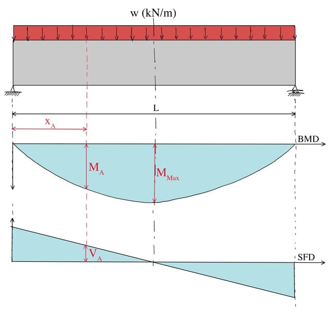
Fig 1. Simply supported beam subject to a uniformly distributed load and the resulting bending moment and shear force diagram.
If we imagine making a vertical cut through our beam at some distance along the length of the beam we can visualise the (linear) normal and (parabolic) shear stress distribution through the depth of the beam at that point, Fig 2. The normal stress distribution, is obtained using the engineer’s bending equation,
where is the bending moment at the location of the cut, is the height from the neutral axis of the beam to the point at which the normal stress is being determined and is the second moment of area of the beam cross-section. The negative sign ensures a negative normal stress is obtained for compression stresses above the neutral axis.
The shear stress distribution is given by the following equation,
where is the shear force at the location of the cut, is the first moment of area of the area above the level at which the shear stress is being determined, is the second moment of area for the cross-section and is the width of the cross-section.
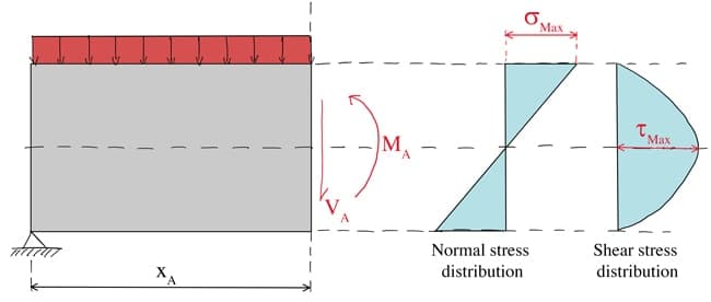
Fig 2. Vertical section through the beam at position and the normal and shear stress distribution down through the depth of the section.
If we now imagine evaluating the normal and shear stress at a height above the neutral axis, we would obtain normal and shear stresses and respectively as shown below. This is where our 2D stress element comes in useful. We can represent the state of stress at this point in the structure on a 2D stress element. To be clear, we are showing the state of stress at location or coordinates on the 2D stress element below.
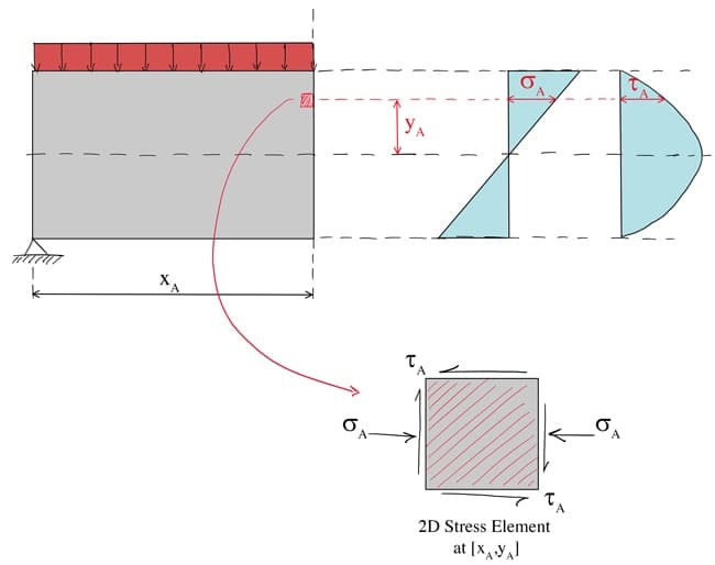
Fig 3. Stresses at horizontal position and at vertical distance from the neutral axis, represented on a 2D stress element.
We talk more about sign conventions for normal and shear stress in video 2, for now it’s sufficient to recognise that the 2D stress element is acting as a ‘stage‘ on which we can ‘display‘ the stresses that exist at this location. The normal stress is shown as a compression stress (squeezing the element) which we typically define as a negative quantity. The shear stress as shown is negative when considered against the sign convention defined in the video – you’ll definitely want to review this video, particularly for when we discuss maximum shear stresses below.
🚨 The big question now is what would happen to the stress magnitudes if we rotated our 2D element?
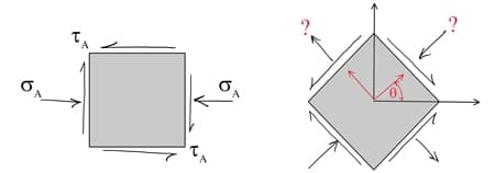
Fig 4. Normal and shear stresses on a 2D stress element (left), unknown stress magnitudes after 2D element is rotated through an angle (right).
The stresses we have shown on our 2D element above are merely the set of stresses that exist on the planes depicted by the 2D stress element i.e. a set of orthogonal planes that happen to be aligned conveniently with the beam. This is not to say that these are necessarily the maximum values of normal and shear stress at that point. There could exist an alternative pair of mutually perpendicular planes, at the same location but at some other orientation, on which the normal or shear stresses will have a larger or smaller magnitude. As engineers, this is clearly something we’d like to know more about! This is where stress transformation equations enter the picture.
3. Stress Transformation Equations
If we know the state of stress at a point on one pair of mutually perpendicular planes, the question we posed in the previous section was, what are the stress magnitudes on other planes of different orientations at the same point? It would make our lives a lot easier if we could determine the normal and shear stresses as a function of the angle of the planes. Fortunately this is exactly what the stress transformation equations allow us to do.
The stress transformation equations can be derived by using simple statics and we cover the process in detail in videos 2 and 3. For now, we’ll simply state the equations and discuss what they’re telling us. We can start by imagining some 2D stress element subject to a normal stress in the horizontal direction, a normal stress in the vertical direction and and shear stress acting on the vertical faces and acting on the horizontal faces.
You’ll recall from the principle of complimentary shear stresses that the magnitudes of the shear stress acting on all faces are equal and that the direction of any one shear stress will define the directions of the three others (such that equilibrium of the element is maintained). We can visualise our stress element below.
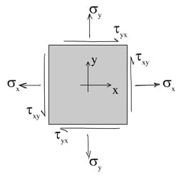
Fig 5. Stress element subject to orthogonal normal stresses and shear stresses.
Now imagine the element rotated counter-clockwise by some angle . When we talk about rotating the element, what we’re really talking about is considering stresses on a set of rotated planes. The axis now denotes the local axis of the rotated element/planes and this axis system is rotationally offset from the original axis by degrees. The normal and shear stresses on this rotated set of planes, , and are shown below.
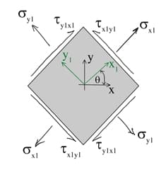
Fig 6. Stress element orientated at angle with respect to the and axis, subject to orthogonal normal stresses and shear stresses.
We can determine the stresses on the rotated set of planes using stress transformation equations (refer to videos 2 and 3 for the derivation),
These three transformation equations allow us to determine the stresses (, and ) on any set of planes provided we know the stresses on a set of planes (, and ) and the angle between the two sets of planes.
At this point we need to make an important observation. If we add the first two transformation equations together, i.e. equations (3) and (4) above, we get the following,
This result tells us that the sum of the orthogonal normal stresses at a point are constant and independent of the angle or orientation of the planes. This is a powerful observation and can be understood by a simple analogy.
Let’s imagine that the state of normal stress at a point could be represented by a single vector and the normal stresses we visualise on our 2D element are just two orthogonal components of that vector. By rotating the planes, we’re merely considering different orthogonal components of the same underlying vector – so the underlying state of stress at that point (the vector in our analogy) is not changing – only the orthogonal components as the reference axis changes. We can visualise this below.
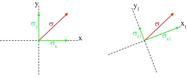
Fig 7. Normal stress components and aligned along axis system (left), normal stress components and aligned along axis system (right). Note the resultant vector is unchanged between the left and right diagrams.
To get a better insight into what the transformation equations are saying, we can plot them. For the purpose of the exercise let’s assume stresses with the following magnitudes,
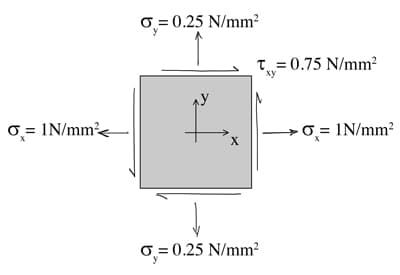
Fig 8. Assumed stresses on the faces corresponding to an orientation of zero degrees.
We walk through the Python code to evaluate the stresses and produce the following plot in video 3. We can clearly see that the stress magnitudes vary sinusoidally. The dashed vertical line at identifies the magnitudes of the three stresses indicated in Fig 8. above at zero degrees. The second dashed vertical line indicates the stresses that would be observed if the the element were rotated by .
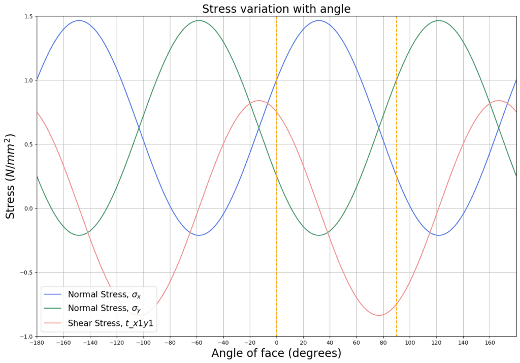
Fig 9. Variation of normal and shear stress with angle
By observing the blue and green lines representing normal stresses and respectively, we can see that their magnitudes are perfectly out of phase with each other – in other words, when one is a maximum, the other is a minimum. On close inspection we can also see that at the angle at which the maximum and minimum normal stresses occur, the shear stress, shown in red, is zero. These are all important results that are discussed further in lectures 4 and 5.
Perhaps the biggest takeaway so far from our plot of the transformation equations is that the stresses we started with, indicated in Fig. 8 are clearly not the maximum values of normal or shear stress that occur at this position in the structure. There exists another pair of planes on which the maximum and minimum normal stresses occur and there are yet another pair of planes on which the maximum shear stresses occur. This observation motivates our discussion of Principal Stresses in the next section.
4. Principal Stresses and Principal Planes
As the name suggests the principal stresses are the maximum and minimum values of the normal stress. These stresses occur on mutually perpendicular planes called principal planes. We can confirm this by observing the peak in the blue line at approximately in Fig 9. This peak denotes the maximum principal stress occurring on a principal plane orientated at to the horizontal axis. If we continue to rotate our element/plane by a further 90 degrees to approximately , we see that the blue line is now at a minimum. This is the minimum principal stress occurring on a principal plane orientated at to the first principal plane.
We can derive a convenient expression for the magnitudes of the principal stresses and the orientation of the planes on which they act, see video 4 for the derivation and further explanation. We can state the key equations here; the principal stresses are given by,
where is the algebraically larger principal stress and is the smaller one. The principal angles are determined from,
The angle has two values, apart. One value identifies the plane on which acts while the other identifies the plane on which acts. Both angles can be substituted into our original transformation equation (Eqn 3.) to determine the principal stress for each angle. The values obtained will agree with the principal stresses obtained using equation 7.
Using equations 7 and 8 we can determine the principal stresses for our example to be and . We also identify principal angles of and . We can plot vertical lines indicating the principal angles and horizontal lines indicating the principal stresses. If we overlay these on our original plot of the transformation equations, we can see that equations 7 and 8 do indeed identify the local maxima and minima, i.e. our principal stresses. From the graph below we can see that the maximum principal stress occurs on the plane oriented at while the minimum principal stress occurs on the plane orientated at .
Equations 7 and 8 are valuable tools as they allow us to identify principal stresses and their orientations provided we know the stresses on any pair of planes. So a typical stress analysis task would be to identify the principal stresses and principal planes at a point by first identifying a more conveniently obtainable set of stresses – like for example the normal and shear stress in the beam at the top of the page.
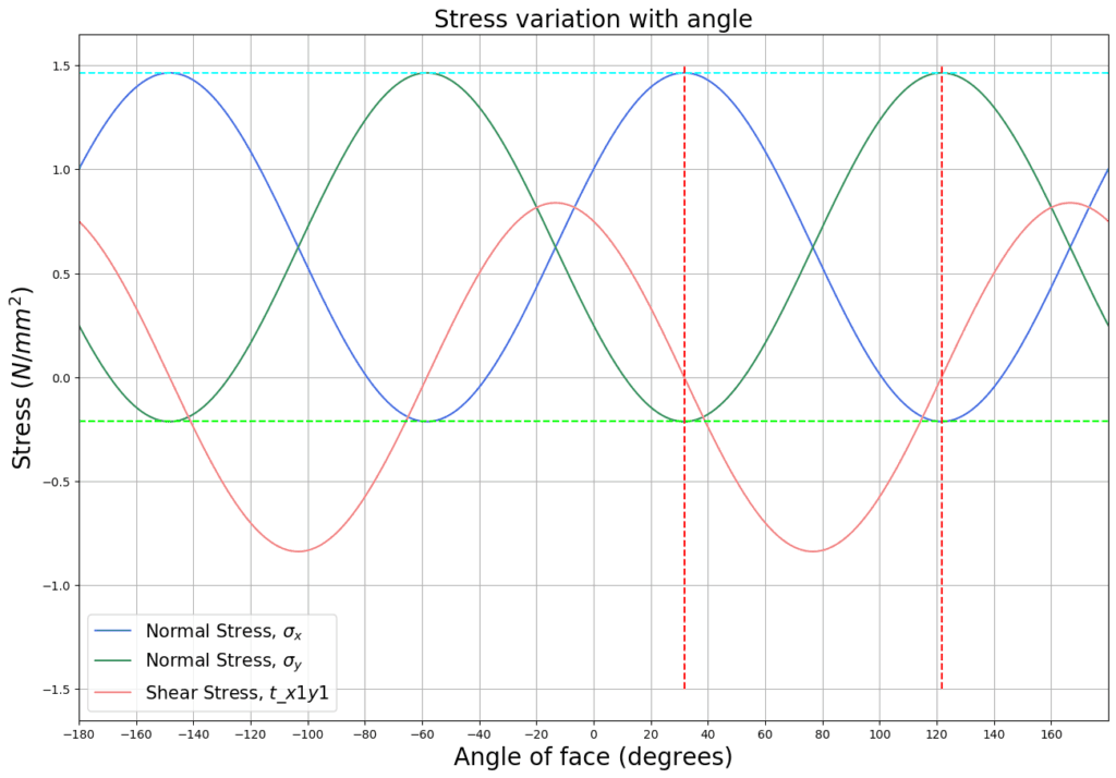
Fig 10. Variation of normal and shear stress with angle. Red vertical lines indicate principal angles identified from equation 8 while horizontal lines indicate principal stresses identified from equation 7.
5. Maximum shear stresses and planes of maximum shear stress
We can now turn our attention to the maximum shear stresses and the planes on which they occur. The reference video for this discussion is video 5. In that video, through a similar derivation process, we show that the maximum shear stress is given by,
and that these stresses occur on planes orientated at to the principal planes,
If we now use equations 9 and 10 we can identify the maximum shear stress magnitude as . The mutually perpendicular planes on which these shear stresses act are orientated at and . We can confirm this graphically by plotting these values on top of a plot of the shear stress transformation equation, Fig 11.
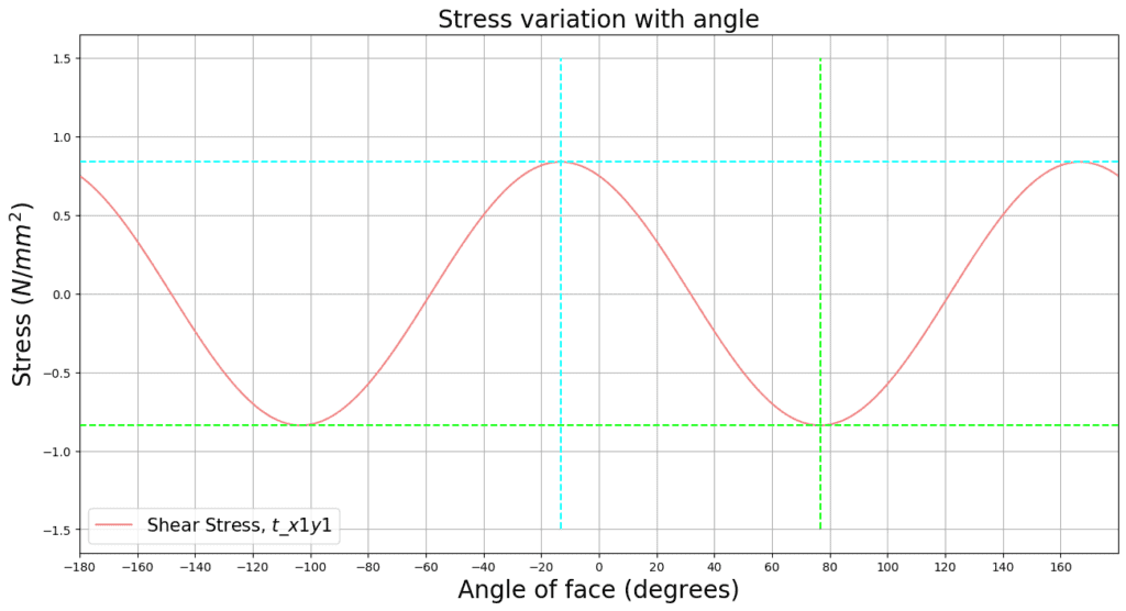
Fig 11. Variation of shear stress with angle with max shear stress magnitude and orientation of planes of max positive and negative shear stress identified.
Before reading the next paragraph, make sure you’ve reviewed the discussion of shear stress sign convention in video 2. With reference to Fig 11. we can see that when the element is orientated at , i.e. when the outward pointing normal from the positive x-face makes an angle of with the global positive x-axis, the shear stress is . However, when the element **(and its reference axis system)**is rotated by , the shear stress acting on the face orientated at is . The change in sign here is because the reference axis for the element has rotated through but all of the shear stress arrow directions remain unchanged. If this last paragraph has totally confused you, make sure to go back and review videos 2 and 5!
6. Mohr’s Circle and Building our Mohr’s Circle Calculator
Now that we have the ground work covered we can introduce Mohr’s circle. As we stated at the outset, Mohr’s circle allows us to capture the complete state of stress at a point in a single graphic. We’ll break this discussion into 2 parts. First we will outline the basic equations; the equation of the circle itself, the radius and the centre of the circle. We’ll also outline the process of building a Mohr’s circle given the necessary starting information. In the second phase of the discussion we’ll use Mohr’s circle to perform an example stress analysis. It’s in solving this example in our Jupyter Notebook that we effectively build our Mohr’s circle calculator.
6.1 Building Mohr’s circle from the transformation equations
The equation of the circle (Mohr’s circle) is derived from the transformation equations. We walk through the process in video 8. Here we’ll summarise the key points. We can show that the equation of the circle is,
where represents the radius of the circle and is given by,
and . If we compare equation 11 to the standard equation of a circle with radius and centre at coordinates ,
we see that the centre of Mohr’s circle is located at coordinates . Now that we know the coordinates of the centre of the circle and the radius, we have enough information to actually build or draw the circle. Since every point on the circle represents the stresses on a particular set of planes – the circle captures the complete state of stress at the point. Let’s assume we know the normal and shear stresses (, and ) on a stress element at a known orientation – say our default orientation where the planes align with the global axis system. From here, the process of actually building and using Mohr’s circle is pretty much the same every time:
- Establish an axis system for the circle where the horizontal axis measures and is positive to the right and the vertical axis measures and is positive downwards.
- Locate the centre of the circle at .
- Locate point ‘A’ on the circle representing the stresses you started with at the default orientation, (, and ).
- Locate a point ‘B’ on the circle which represents the stresses on the adjacent perpendicular face of the element. Point ‘B’ will therefore have coordinates () on the circle.
🚨 It’s important to note that a rotation of degrees on our 2D stress element corresponds to a rotation of around Mohr’s circle.
6.2 Mohr’s Circle Example
Now we can put Mohr’s circle to use and complete an example stress analysis. We’re going to implement our calculations and plot the Mohr’s circle for this analysis in our Jupyter Notebook. The beauty of coding this is that once complete we will have built a Mohr’s circle calculator! The process is covered in video 9. I’ll briefly discuss the output of our analysis here. We start with a candidate question to answer; consider the following 2D stress element subject to the stresses shown.
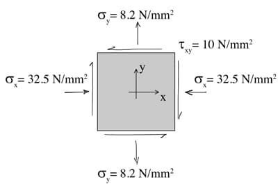
Fig 12. 2D stress element subject to normal and shear stresses.
The first task is to work out to identify the centre of the circle and then to calculate the radius of the circle,
Now we can draw the circle, or plot it using Python in our case and immediately identify the principal stresses, maximum shear stresses and their associated planes.
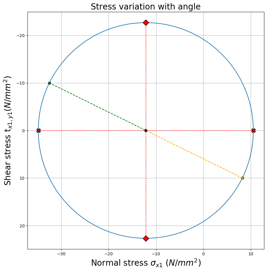
Fig 13. Mohr’s circle showing the principal stresses (red crosses), maximum positive and negative shear stresses (red diamonds), stresses on the planes depicted by the 2D stress element in Fig 12. above (green dot for face and yellow dot for face)
We can see that the principal stresses can be identified from knowledge of the circle centre and radius,
Similarly the maximum positive and negative shear stress is simply .
The angles of the principal planes and the planes of maximum positive and negative shear stress can be easily identified using basic trigonometry and using the green dashed line as the reference line that represents i.e. the orientation of the element shown in Fig. 12. Just remember that an angle of on Mohr’s circle corresponds to a rotation of degrees on our element. The fact that our vertical axis is positive downwards also means that the sense of rotation of the element matches the sense of rotation on our circle, i.e. a counter-clockwise rotation of the element by degrees corresponds to a counter-clockwise rotation of degrees from our reference axis on the circle (green dashed line in our case).
As I’ve said – the beauty of building this solution using Python in our Jupyter Notebook (video 9) means that simply by changing the input parameters, i.e. the stresses shown in Fig. 12, we can automatically generate the corresponding Mohr’s circle from which we can then determine the stresses at any orientation.
So there you have it – we’ve covered everything from the basics of normal and shear stress all they way up to Mohr’s circle. If you’ve been following along and watched the videos series accompanying this post, you’ll also have built yourself a handy Mohr’s circle calculator. Aside from developing knowledge of the underlying theory – the real win with this project is that you should feel confident enough to start tinkering with your code and making additions to build a stress analysis calculator that suits you.
Now you’ve seen how we can automate a standard engineering calculation – what other repetitive calculations can you automate? Why not start building your own library of analysis notebooks?!
If you want to dive deeper into stress analysis and build your own finite element analysis code, take a look at the course abovebelow. In that course, you’ll put the knowledge and coding skills you picked up here to good use and build a complete 2D finite element analysis tool, right inside another Jupyter Notebook!
Finite Element Analysis of Continuum Structures in Python
Use the Isoparametric Finite Element Method to build an analysis tool for 2D structures in Python.
After completing this course...
- You will have the tools to analyse continuum structures using your own Isoparameteric Finite element Python code, developed from the ground up.
- You will understand how the assumptions of plane stress and plane strain allow us to analyse 3D structures accurately with 2D planar models.
- You will be able to use open source tools to generate structural models and mesh data that can be analysed with your FE code.
That’s all for this one – see you in the next one. 👍
Dr Seán Carroll's latest courses.


Featured Tutorials and Guides
If you found this tutorial helpful, you might enjoy some of these other tutorials.
Plate Girder Design to Eurocode 3
A step-by-step guide to the design of code-compliant steel plate girders.

Callum Wilson
An Introduction to form-finding with Thrust Network Analysis
A powerful form-finding method for compression-only shell structures and masonry vaults.

Oliviero Cabitza
A Structural Modelling and Analysis Addon for Blender [RELEASED]
You can now download the complete StructureWorks addon!

Dr Seán Carroll


![A Structural Modelling and Analysis Addon for Blender [RELEASED]](/_next/image?url=%2Fimages%2Fposts%2Fa-structural-modelling-and-analysis-addon-for-blender%2Fa-structural-modelling-and-analysis-addon-for-blender.jpg&w=1200&q=75)