Influence Lines - A Complete Introduction for Civil and Structural Engineers
![[object Object]](/_next/image?url=%2Fimages%2Fauthors%2Fcallum_wilson.jpg&w=256&q=75)
Welcome to this tutorial on influence lines. In this tutorial, we’ll develop an understanding of influence lines for determinate and indeterminate beam structures.
By the end of this tutorial, you will be confident in constructing influence lines for determinate structures. You will also develop an appreciation of how we can implement more advanced structural analysis techniques to construct influence lines for indeterminate structures.
All Access Membership
Learn, revise or refresh your knowledge and master engineering analysis and design
Access Every Course and Tool
- Over 1140 lectures & over 234 hours of HD video content
- Access member-only 'deep dive' tutorials
- Access all downloads, pdf guides & Python codes
- Access to the StructureWorks Blender addon + updates
- Packed development roadmap of courses & tutorials
- Price Guarantee – avoid future price rises as we grow
- Priority Q&A support
- Course completion certificates
- Early access to new courses
1.0 What is an influence line?
An influence line is a graphical representation of the variation of some chosen action (reaction, shear, bending moment) which occurs in a structural element. The influence line is defined in terms of the position of a unit concentrated dimensionless load , which can occur at any point on the structural element.
This definition is perhaps a little confusing….let us break it down:
- ‘an influence line is a graphical representation’…..ok so we’re expecting either a curve or a straight-line graph, which we know has two variables. The first is the distance along the beam and the second is some dimensionless factor.
- ‘representation of the variation of some chosen action (force, shear, bending moment)’…ok so we’re familiar with a graph which shows the variation of shear force and bending moment along a member, right? But what about reactions? We don’t typically draw a plot for this.
- ‘in terms of the position of a unit concentrated dimensionless load ‘…this should give you a clue! We have the freedom to move the load to any position along the beam, think about why we might want to do this?!
2.0 Why are we interested in influence lines?
Before you clicked on this tutorial and began to think about influence lines, you will have encountered many examples where you have been asked to analyse a beam structure subject to a set of loads. Using our set of statical analysis techniques, we define the reactions, shear forces and bending moments in this structure…great!
In some cases, this approach is sufficient because we can be confident (using engineering judgement) that the applied loads are not going to change their point of application. For example, a column situated at the mid-span of a transfer beam is not going to move!
However, we can quickly think of cases where there is a potential for the position of a load to move to different positions along the structure. When might this occur in the real world?
Without a doubt, the best example is a bridge structure. Vehicles, trains and pedestrians can all move over a bridge, and as they move, the internal forces and reactions of the structure will change. So if we used our traditional approach of calculating a single set of reactions, a single shear force diagram and a single bending moment diagram, how would we know that we had captured the worst case scenario i.e. the largest reaction magnitude and the largest shear force and bending moment?
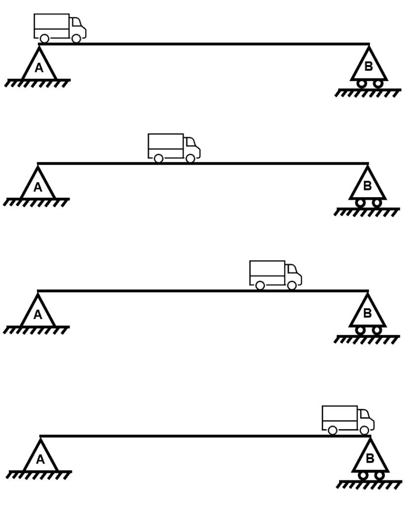
Figure 1. Moving load across a beam structure
Well one approach would be to manually move the position of the applied loads along the structure and then re-calculate the reactions and internal forces, compare them to the previous values and then continue this iterative process until we find the critical values….you can already imagine how time consuming and inefficient this might be!
So, the key idea regarding influence lines is to be able to determine the worst case scenario for a given action by changing the position of load application. This is important because we must ensure that our structures are designed to resist the most adverse loads that they can possibly experience.
Very important note: within this tutorial there will be references to ‘moving loads‘. We must be very clear before proceeding; ‘moving load’ refers to the notion that the position of the load is arbitrary. In our study of ‘moving loads’, we are not taking into account the dynamic effects associated with, for example, a train moving across a bridge…..this is a whole different topic which is outside the scope of this tutorial! Take a look at the EngineeringSkills dynamics courses here and here if you want to explore structural dynamics in more detail.
3.0 Determinate vs Indeterminate Structures
As usual, we can group structures depending on whether they are statically determinate or indeterminate.
There are two common methods to define the influence line for a structure, and our choice depends on whether the structure is determinate or indeterminate. As a summary:
- If the structure is determinate, then we will use the static method and the resulting influence line will be a 1st order polynomial.
- If the structure is indeterminate, then we will use the kinematic method and the resulting influence line will be, as a minimum, a second order polynomial.
We can of course use the (more versatile) kinematic method to analyse simple determinate structures, but it is often handy to have the (less powerful, but) simpler, static method available too!
4.0 Static Method for Determinate Structures
Before we start, let’s remind ourselves exactly what our objectives are….
We want to define a graph (itself described by a function) which can be used to tell us the value of a force or action component (reaction, shear force or bending moment) in terms of the position of the applied load along the structure.
Let’s start with an example.
4.1 Static Method Example: Simply supported beam
Consider the beam in Figure 2 below:
- The beam is simply supported and therefore statically determinate.
- We can apply the point load at any point along the beam so .
- We want to obtain influence lines for the reactions at and .
- We also want to obtain influence lines for the shear force and bending moment at reference point .
- We will say that
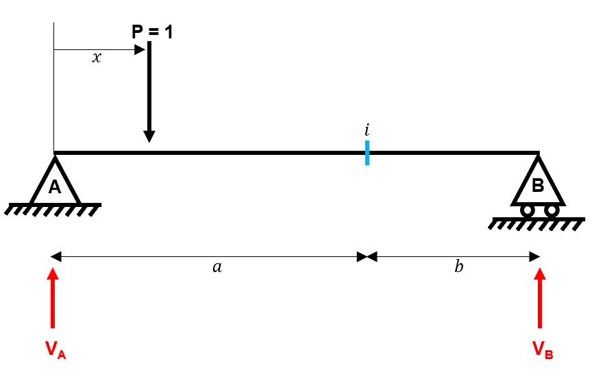
Figure 2. Example 1 general arrangement
4.1.1 Influence line for reactions
Influence line for
We start by following our standard approach for calculating the reactions for a simply supported beam. Importantly, however, we describe the position of the load along the beam using the variable .
Since , then (1) becomes the function describing our influence line which we write as:
Note: is the greek letter ‘iota’ which we use to show that this function is an influence line for the force component .
Ok, so let us plot
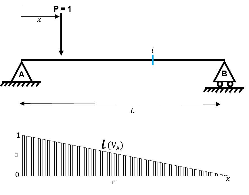
Figure 3. Plot of
We should always conduct a few simple checks to ensure that our function is correct:
-
if we apply the point load at then , which is what we would expect as there can’t be any reaction at if the point load is applied directly over .
-
if we apply the point load at then , which is what we would expect as the maximum reaction at will occur when there is zero reaction at .
Initially, it can be confusing to see influence line diagrams for reactions, especially if you haven’t encountered these in your previous studies of beam analysis. We must remember that the influence line is only telling us about the magnitude of , and not .
The benefit of obtaining the influence line is that if I now told you that the value of the load was 1000kN then all we would need to do is multiply the value of by 1000 to obtain the reaction for any position of the load .
Influence line for
A similar method is used for ….before we start can you guess what the influence line will look like? How is it related to ?
Since , then (3) becomes the function describing our influence line which we write as:
Ok, so let us plot
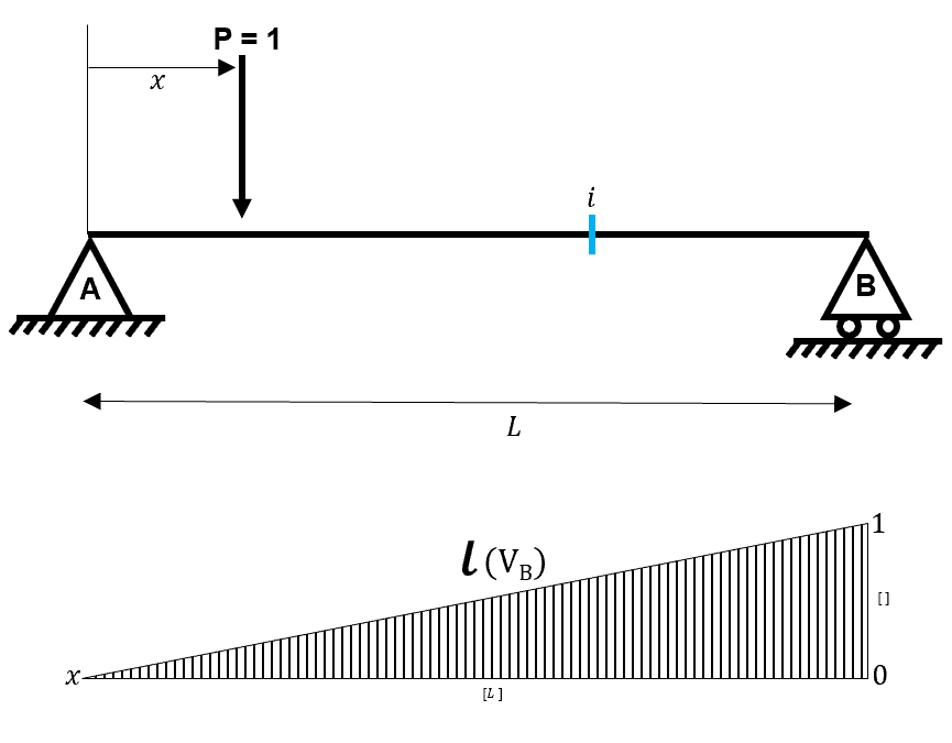
Figure 4. Plot of
Again, let us make a sanity check:
-
if we apply the point load at then which is what we would expect as the maximum reaction at will occur when there is zero reaction at .
-
if we apply the point load at then which is what we would expect as as there can’t be any reaction at if the point load is applied directly over .
Not only this, but we can see that the two influence lines are symmetrical about a point…how can we find this point and what does it mean?
Well, let us set and solve for .
So the two influence lines are equal when .
If we input into (1) and (3) then we get
And this should not be a surprise!
If we apply a point load P at the mid-point of a simply-supported beam, then the two vertical reactions are both equal to ...we have seen this hundreds of times in beam analysis examples. In this example, we have just arrived at the solution in a different way!
4.1.2 Influence line for bending moments
Now let us consider the internal forces.
Influence line for
Before proceeding with the influence line for bending moments at , let us think about how we would approach the analysis of a simply supported beam subject to a point load.
We want to determine the bending moment at …
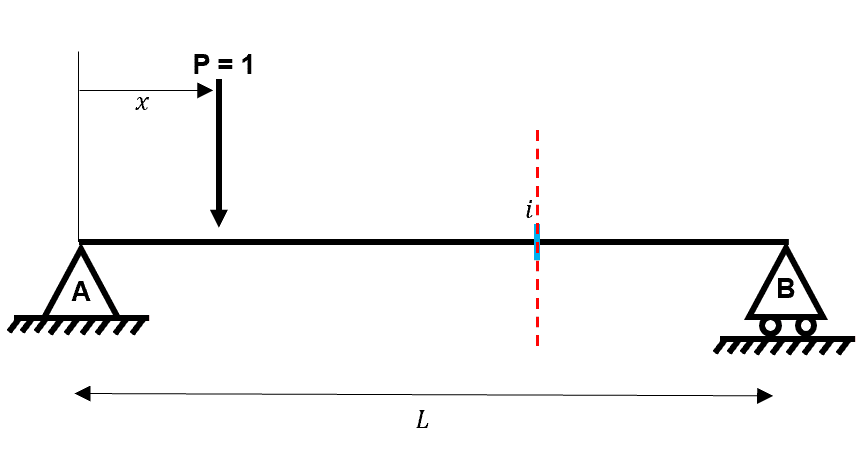
There are two different ways to determine the bending moment diagram at , corresponding to a cut which exposes the left and right-hand side of the beam, respectively.
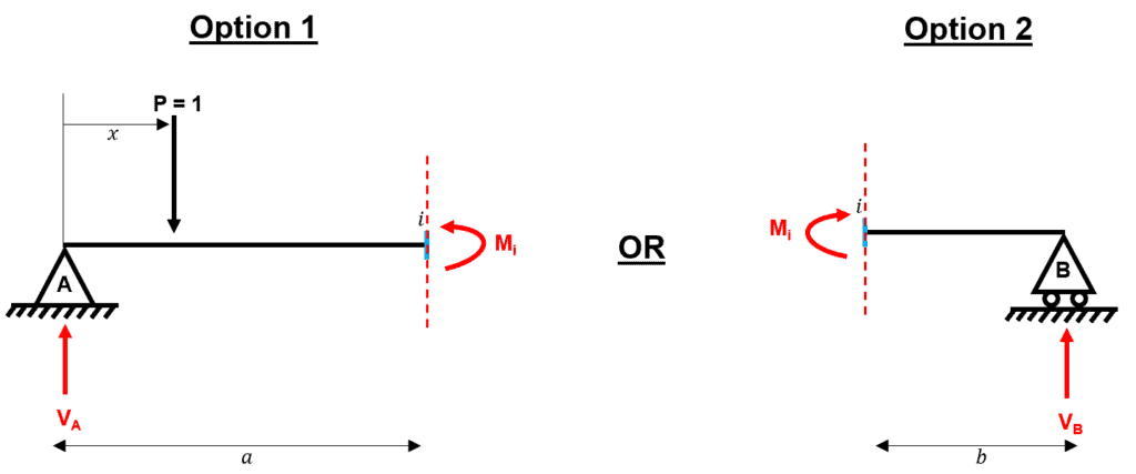
Figure 6. Different options for the cut
Let us assume that we have picked option 1, how would we proceed?
Well, we would consider moment equilibrium about point and this would tell us . Ok, now let us say that we move the position of the point load slightly towards …what happens to the moment …well it changes!
Ok, so we repeat the process for the new position of , this gives us a new …great! Now let us say that we move the position of the point load towards ….you get the idea, we have to repeat the moment equilibrium calculation for each position of .
Now let us consider if we chose to use option 2….can you think why this might be advantageous for us? (Hint: think about the influence lines for reactions we calculated above!)
Using option 2, the moment is simply equal to …but what happens if we move the load …well we already know this!
In the first part of this example we determined which tells us how the value of changes depending on the position of …so how can we use this to determine the influence line for ?
In fact it is rather intuitive…
But we must note that the above is only true for which is applied at
So what happens when is applied to the right side of ….well we use the same logic as above but with the reaction .
and as I’m sure you’ve already noted, this influence line is only valid for applied at
Let us think about our two influence lines graphically.
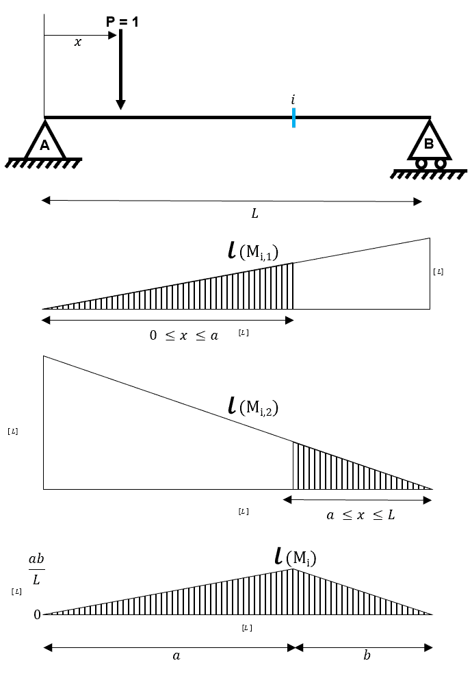
We can see that the two influence lines have the same value at , which is
The final influence line is a piecewise linear function, which we can write as
4.1.3 A quick note on units!
Does an influence line have units? Let us check!
From the equations for and we can see that these influence lines are dimensionless i.e. ..
But for , the units must be [L]
Does this make sense?
We can show that this makes sense by developing our understanding of the use of influence lines!
If I asked you to calculate the bending moment at you might quickly reach for the standard formula of
But now, equipped with the influence line , we can arrive at the same formula for the bending moment at by simply multiplying the value of the influence line at by the load
which in terms of units is which we know is a bending moment!
Influence line for
We approach the influence line for shear force in a similar way to that of bending moment.
For shear force, we consider the equilibrium of vertical forces about a cut at .
Firstly we will consider the case when is applied to the left of . In this case, is simply equal to . If you are not sure how we reached this result then check out the statical derivation below!
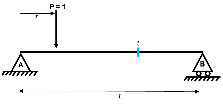
Depending on our preference, we can take equilibrium using option 1 or option 2 below.
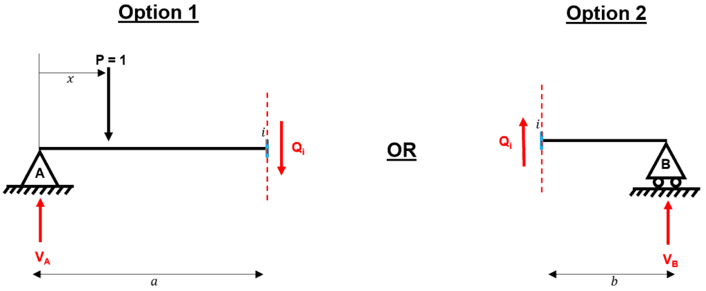
Figure 9. Different options for taking equilibrium at a cut.
If we choose option 1, then
If we choose option 2, then
Again, we know the variation of as the load moves so we can write the following
But again, we must note that the above is only true for , which is applied at
When is applied to the right side of ….well we use the same logic as above but with the reaction .
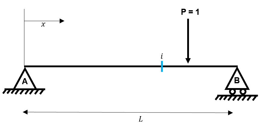
Depending on our preference, we can take equilibrium using option 1 or option 2 below.
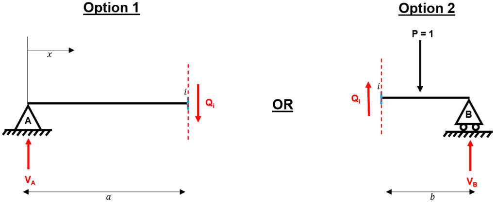
Figure 11. Different options for taking equilibrium at a cut
If we choose option 1, then
If we choose option 2, then
Now, keep the above bounding results in mind whilst we produce a plot of the influence lines for .
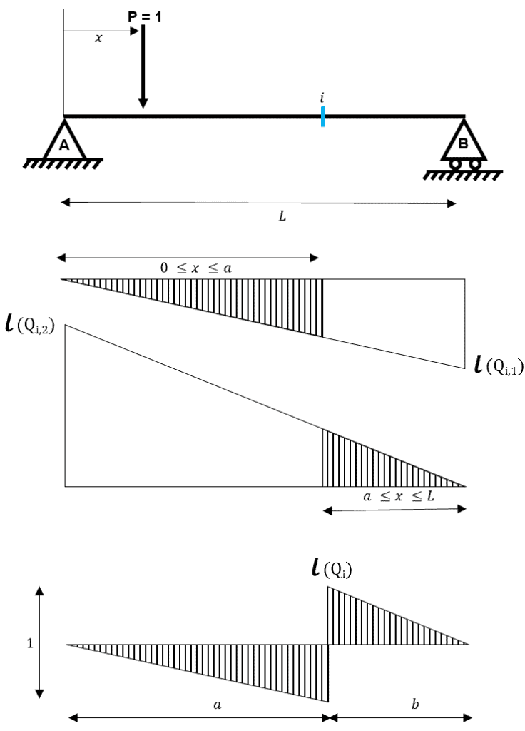
The final influence line is a piecewise linear function, which we can write as
So we have looked at the application of the static method to a very simple statically determinate beam. Let us reflect on the static method!
To conduct the static method, we are essentially generalising a static analysis by describing the position of the load using the variable . Within the static method, we are still using the fundamental methods of force and moment equilibrium but we are using these to determine expressions for influence lines.
We have also discussed that the static method can only be used on determinate structures. In practice, we rarely see determinate structures, and therefore, the static method is arguably of little practical use. The reason it is included here, however, is because it is an excellent way to introduce the meaning of an influence line. Considering the simple example above, you can see that even with the addition of a uniformly distributed load, the descriptions for the influence lines would become significantly more complex.
5.0 Kinematic Method for Indeterminate Structures
So, we concluded the previous section by stating that the static method is of little practical use because (a) it can only be used on determinate structures and (b) to perform the method, we essentially have to complete a generalised static analysis of the element (which is time-consuming for large structures with multiple applied loads).
Before presenting the kinematic method, we must introduce and understand two fundamental results from structural mechanics. These may seem very ‘theory-heavy’, but they are the foundations for determining influence lines using the kinematic method. In fact, these two results can be considered two of the most important results in linear structural mechanics.
5.1 Maxwell’s Reciprocal Theorem
Maxwell’s Reciprocal Theorem is the first result which we need to introduce. We introduce this result first because it is used in the derivation of the second result.
To unpack Maxwell’s Reciprocal Theorem we must familiarise ourselves with influence coefficients. An influence coefficient describes the displacement, in some direction , caused by the application of unit load, in some direction .
In general, an influence coefficient is written as:
Maxwell’s Reciprocal Theorem tells us that in a linear elastic structure, the displacement, in a particular direction, of point due to a load at point will be equal to the corresponding displacement caused at point by the same corresponding load at point …..lots of words right??!….stated more elegantly…
Don’t believe me? Here’s the proof using Virtual Work Principles.
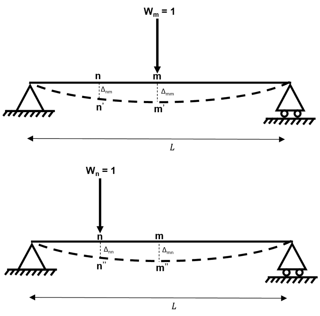
Figure 13. Setting up the proof of Maxwell’s Reciprocal Theorem
So, if is applied to our structure first then the work done by is:
And then, if we apply subsequently then the work done by is:
But we must recognise that due to the application of , the structure has deformed beyond the deformed shape due to the earlier application of and hence additional work is done by . This additional work is given by:
We can now consider the total work done by the two loads and this allows us to define the strain energy stored in the structure.
Great! You are probably wondering what this is telling us….
Ok, now let’s start all over again and instead apply before …skipping all of the repeated algebra from the previous lines we arrive at
Now, from the Principle of Conservation of Energy we know that and therefore:
and hence:
And there we go, we have demonstrated Maxwell’s Reciprocal Theorem!
You are probably still asking why we are delving into all of this theory! Well, stick with me; all will become clear.
5.2 Müller-Breslau Principle
The second fundamental result for us to introduce is the Müller-Breslau Principle.
Consider the indeterminate beam example below, let us say that we want to determine the support reaction at point B due to a unit vertical load at location X.
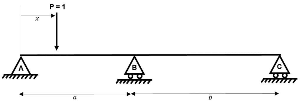
Figure 14. Example problem to demonstrate the Müller-Breslau Principle
To determine this reaction we develop an auxiliary determinate system in which the support B is removed and the support reaction is replaced with an unknown load. We also invoke Maxwell’s notation to indicate the influence coefficients at each point.
From compatibility requirements we know that and that:
Graphically, the compatibility system is as below:
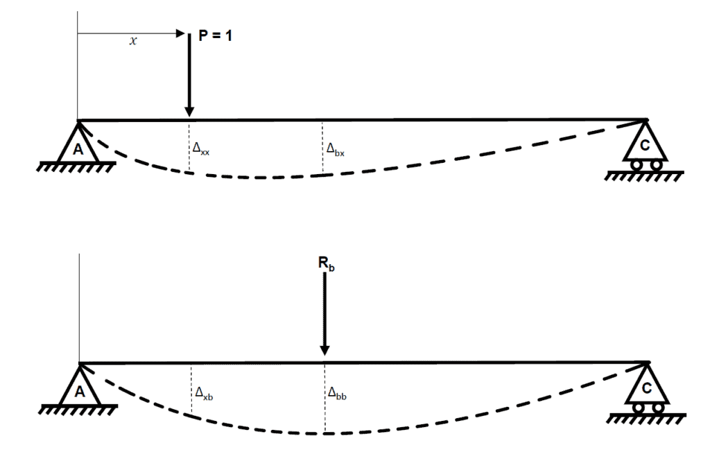
Figure 15. Elastic deformation of the system
Now, using the influence coefficient notation.
Giving the support reaction at B due to a unit load at location X as:
Ok, let’s slow down for a second….
We have just determined an expression for the ‘support reaction at B due to a unit load at X’. Think back to what we did in the static method presented earlier….we were doing exactly the same. We were placing a unit load at position X and developing an expression for the support reactions. Ok, so you should be able to see how the kinematic method is developing. Let’s develop this idea further.
Firstly we can employ the result of Maxwell’s Reciprocal Theorem whereby:
and therefore
The above expression is actually an expression for the influence line for the support reaction . But in reality this expression isn’t much use because the influence line is expressed in terms of influence coefficients, which themselves are defined in terms of displacements caused by a unit load.
It would be more useful if we could express the influence line in terms of the deformation alone. So we consider the following:
And since:
and
We get,
Now, here comes the important step. If we set i.e. a unit displacement at B, then we arrive at:
So now we can revisit our expression for the influence line and say that:
In other words, we can say that the ordinate of the influence line for the reaction at B is proportional to the negative ordinate of the deformed shape of the system when a unit displacement is applied at the released degree of freedom corresponding to the location and force quantity we are interested in.
5.3 Implementing the Kinematic Method
We now have an understanding of how we can use the Müller-Breslau Principle to define the influence line for a required force quantity. In simple terms, to define the influence line for a given quantity at a given location, we need to define the ordinates of the elastic deformation at that point due to a unit displacement applied at that same point. The kinematic method can be used for determinate or indeterminate beam structures.
Let us implement the theory by considering a determinate example.
5.3.1 Kinematic Method Worked Example: Simply Supported Beam
Wait...didn’t we discuss the fact that the kinematic method is used for extremely complicated indeterminate beams?!
Well, yes it CAN be used to analyse indeterminate beams but it can also be used to analyse determinate beams. In my experience, it is always sensible to reproduce results from a simple method (the static method) using a more complicated method (the kinematic method) to ensure that everything checks out!
With that in mind, we will repeat the Static Method Worked Example to demonstrate that we can obtain the same results using both methods!
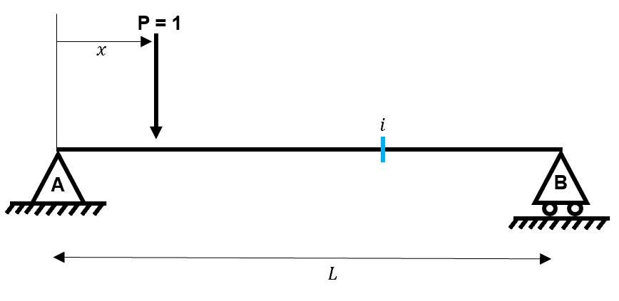
Figure 16. General arrangement of the worked example
Influence line for
We simply release the necessary degree of freedom at the point of interest and apply a unit displacement so that the structure performs negative virtual work.
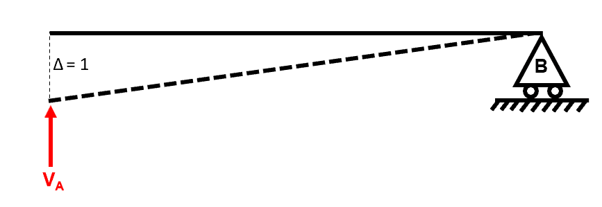
Figure 17. Deformed geometry of the structure due to unit displacement at A
We recall the conclusion that the ordinate of an influence line is proportional to the negative ordinates of the deformed shape of the system when a unit displacement is applied at the released degree of freedom corresponding to the location and force quantity we are interested in. Therefore, if we mirror the deformed geometry in figure 17 then we arrive at the influence line for .
You should recognise this plot as it is identical to figure 3! This proves that both the static and kinematic method result in the same influence line.
Influence line for
Again, release the necessary degree of freedom at the point of interest and apply a unit displacement so that the structure performs negative virtual work.
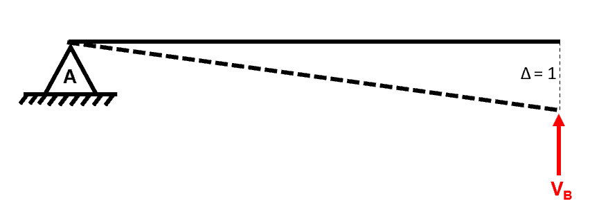
Figure 18. Deformed geometry of the structure due to unit displacement at B
Again, if we mirror the deformed geometry, then we arrive at the influence line for . We note that this plot is identical to figure 4.
Influence line for
Following the same method, we release the degree of freedom associated with bending at position by invoking a hinge. We then apply a unit displacement (rotation) at so that the structure performs negative virtual work.
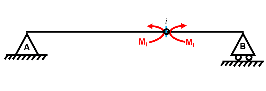
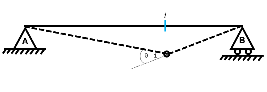
Figure 20. Deformed geometry of the structure due to unit rotation at
To obtain the influence line we simply mirror the deformed elastic geometry due to the applied unit displacement. Does this influence line plot match figure 7 (obtained using the static method)? Yes it does!
Influence line for
For the shear force, we have to introduce a new type of hinge – we refer to it as the sliding hinge. The sliding hinge is necessary as we need to develop negative virtual work via shear force only (and not via bending moments). For this to be the case, there can be no rotation at the sliding hinge.
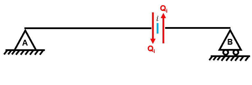
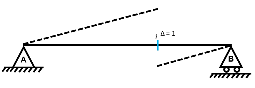
Figure 22. Deformed geometry of the structure due to unit sliding displacement at
Following the kinematic method we now mirror the deformed elastic geometry which allows us to extract the influence line. Again, we check that this matches our result from the static method in figure 12!
6.0 Using the Kinematic Method for more complicated examples
We have demonstrated the theory of the kinematic method using a very simple determinate example. We were able to complete this example very quickly because it is not difficult for us to draw the deformed shape of a single span simply supported beam due to a unit displacement.
However, to apply the kinematic method to more complicated determinate or indeterminate structures, we need to be able to define the deformed shape of the structure under unit displacements at points of interest.
Ultimately, therefore, the problem of defining the influence line simplifies to the problem of defining the deformed shape of a structure due to a unit displacement at a specific point, with a specific degree of freedom released.
7.0 Conclusions
Hopefully, you’ve now gained an appreciation for why influence lines are a valuable tool for the Civil and Structural Engineer. In many practical applications, it is important for the Engineer to be able to define the worst case scenario for internal forces and reactions.
Two different methods have been introduced:
- the static method
- and the kinematic method.
The static method can only be used for determinate structures and as a result, is of limited practical value.
The kinematic method is the preferred method and can be used for determinate and indeterminate structures. The kinematic method is a powerful approach which relies upon two governing results from linear elastic mechanics and involves defining the deformed shape of the structure under a unit displacement.
Several analysis techniques can be used to define the deformed shape of a structure under a unit displacement, but the direct stiffness method is considered to be an appropriate choice because it gives us the ability to quickly release degrees of freedom at nodes of our choice.
So that’s it for this tutorial, I hope you found it interesting and helpful. The theory of influence lines is not always immediately intuitive but they are an extremely important tool in structural engineering!
Featured Tutorials and Guides
If you found this tutorial helpful, you might enjoy some of these other tutorials.
Truss Analysis using the Method of Joints and Method of Sections
Using the method of sections and method of joints to work out the internal forces in statically determinate trusses

Dr Seán Carroll
Steel Truss Design to Eurocode 3
Learn how to design one of the most common structural forms - the steel truss

Callum Wilson
Column Buckling Equations
Determine column buckling equations for axially loaded column with different end conditions

Dr Seán Carroll

