A Pynite Crash Course - Open Source Finite Element Modelling for Structural Engineers
![[object Object]](/_next/image?url=%2Fimages%2Fauthors%2Fdan_ki.png&w=256&q=75)

Welcome to another EngineeringSkills tutorial! This time, our man in New York, Dan Ki, is back with a fantastic introduction to Pynite. This is an open source finite element analysis library that just reached version 1.0 and is ready for prime time! So, it's a great time to dive in and learn how to use it.
Dan walks us through the analysis of three example structures and then finishes up with a real-world case study that combines Pynite with another open source library - sectionproperties. This is a great way to get hands-on with Pynite and see how it can be used in practice.
When you've finished this tutorial, you can read part 2 which covers the analysis of plate structures using Pynite, here.
Tutorial breakdown
📍 1.0 Is commercial software always the best option?
Why should we bother getting to know these open source libraries? Don't we generally have fully featured commercial software at our fingertips? Dan makes a great case for why we should all be getting to know these libraries and how they can help us in our day-to-day work.
📍 2.0 Introducing Pynite - open source finite element modelling
In section 2 we get a quick introduction to Pynite and its capabilities. We also take a high-level overview of how Pynite is structured and how we can use it to build our models.
📍 3.0 Example 1 - Simply supported beam
Every good programming intro needs a 'Hello World' example! If you're a structural engineer - this is undoubtedly a simply supported beam. So, to get us started with Pynite, we build and analyse a simply support beam subject to dead and live distributed loads.
📍 4.0 Example 2 - 2D frame
In section 4 we turn our attention to 2D frames - probably the type of structure you'll use Pynite for most often. This example comes from a validation set provided by CSI, and it's one Dan regularly uses to benchmark any new FE software he works with - having a go-to validation structure is always a good idea when testing new tools!
📍 5.0 Example 3 - 2D truss (the old reliable)
With 2D beams and frames covered, we shouldn't really move on without covering 2D trusses. For this example, we return to an EngineeringSkills favourite (my typical truss validation structure) - the inverted bowstring truss. This will give us the chance to demonstrate how degree of freedom releases are implemented.
📍 6.0 Example 4 - Real-world case study
In the final example, Dan draws from his own consultancy experience and presents a real-world case study. Although the structural problem being addressed is relatively simple, it's a great example of how we can use open-source tools to quickly work up a solution and explore alternatives. In this example, we combine Pynite and SectionProperties - two libraries that work great together!
📍 7.0 Conclusion
In section 7, we wrap up with some concluding thoughts on the power and utility of open source tools and why the modern engineer shouldn't be afraid to get their hands dirty with a little programming!
I hope you enjoy the tutorial - I certainly did!
📂 Make sure to download the Jupyter Notebook (linked above) to run locally as you read through the tutorial.

1.0 Is commercial software always the best option?
In structural engineering practice, there is often a tendency to default immediately to commercial software when tackling simple design tasks. For example, when tasked with designing a set of multi-span continuous transfer beams, many engineers instinctively rely on sophisticated software such as SAP2000. While SAP2000 performs effectively, it may not always be the most efficient choice (especially in offices with limited licenses).
There is certainly a time and place for commercial software, particularly for complex analyses that require advanced features, detailed visualisation and verification. Engineers should be capable of discerning when commercial software is appropriate and when simpler, more streamlined alternatives might suffice.
Fortunately, alternative solutions exist that are free, efficient, and require only basic programming knowledge to implement. Leveraging open-source libraries can sometimes offer a powerful and accessible alternative to commercial software, encouraging structural engineers to become proficient in programming languages such as Python or C#. It is increasingly evident that programming, ranging from simple scripting to developing comprehensive libraries, will become a requisite skill for structural engineers moving forward.
If you're given a hammer, everything looks like a nail.
As the saying goes, "If you're given a hammer, everything looks like a nail". Rather than relying on a single tool, it is beneficial to expand your engineering toolbox with diverse options. In my previous tutorial here on EngineeringSkills, we saw how we can streamline the analysis of reinforced concrete columns using concreteproperties. Now, we'll introduce another powerful addition to your engineering toolbox - Pynite.
2.0 Introducing Pynite - open source finite element modelling
This introductory tutorial is the first part in our multi-part series on Pynite, an open source Python FEA library by Craig Brinck. Right off the bat, let's take a quick peek at Pynite's capabilities.
- 3D static analysis of elastic structures.
- P- analysis of frame type structures.
- Member point loads, linearly varying distributed loads, and nodal loads are supported.
- Classify loads by load case and create load combinations from load cases.
- Produces shear, moment, and deflection results and diagrams for each member.
- Automatic handling of internal nodes on frame members (physical members).
- Tension-only and compression-only elements.
- Spring elements: two-way, tension-only, and compression-only.
- Spring supports: two-way and one-way.
- Quadrilateral plate elements (DKMQ formulation).
- Rectangular plate elements (12-term polynomial formulation).
- Basic meshing algorithms for some common shapes and for openings in rectangular meshes.
- Reports support reactions.
- Rendering of model geometry, supports, load cases, load combinations, and deformed shapes.
- Advanced tools for modeling and analysing complex shear walls.
- Generates PDF reports for models and model results.
As you can see, Pynite has a wide-ranging, impressive set of capabilities, which is very exciting! Although I have used Pynite for simple 2D analyses, I have been hesitant to build a full workflow around Pynite due to it being in a beta version.
However, Craig has recently pushed Pynite to its first major version (thank you, Craig!). Since this means that we, as users, can expect a more stable API, I've become sufficiently motivated to explore Pynite more seriously and perhaps incorporate it into my design workflows.
However, my goal isn't to build complicated 3D models or perform detailed P-Delta analyses (although Pynite is capable of this) - commercial software is generally better suited to handle those tasks more effectively. Instead, I view Pynite as a valuable addition to my engineering toolkit, ideal for automating or speeding up simple or tedious design tasks.
It also serves as an excellent academic tool, helping us build intuition and enhance our engineering judgement by quickly providing initial insights into structural behaviour. Understanding the strengths and limitations of our tools is essential, and Pynite shines in giving us a solid starting point for more detailed analyses.
2.1 Pynite's internal structure
Before we start coding, it will be helpful to develop a mental model of how Pynite is organised. At the heart of Pynite is the FEModel3D() class, which acts as a container for almost everything in the finite element model.
Everything branches out from this core class - nodes, members, supports, loads, solution algorithms, post-processing, etc. Think of instantiating FEModel3D() as opening a blank model in your favourite commercial software. Figure 1 below shows a high-level (and non-exhaustive) component diagram. The only thing not directly handled by FEModel3D() is reporting and rendering, which are handled by separate modules (we'll discuss this more down the line).
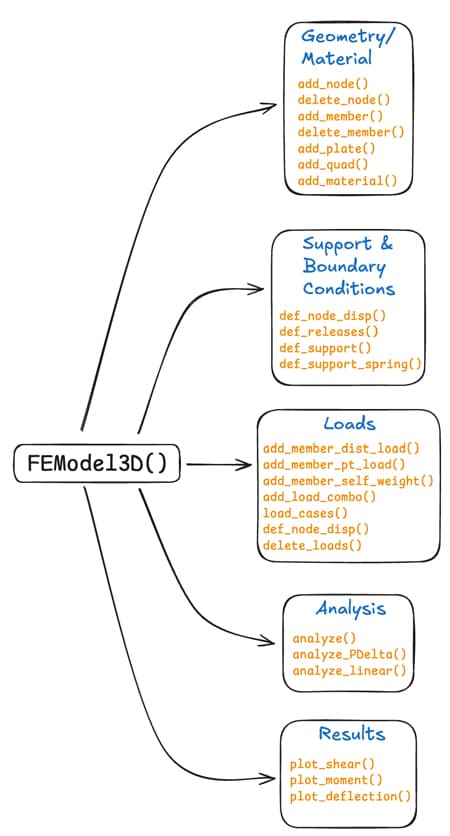
Fig 1. Non-exhaustive component diagram of Pynite's internal structure.
2.2 Coordinate system and units
As with any structural modelling toolset, it's critical to understand the local member coordinate system employed. Figure 2 below (sourced from the Pynite github repo) illustrates the local coordinate system used in Pynite.
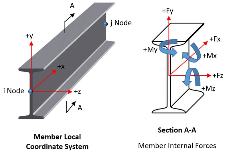
Fig 2. Local member coordinate system used by Pynite, [Source].
Lastly, Pynite is agnostics to units, meaning it does not enforce any specific unit system - this is a good thing! However, this requires careful consistency; whatever units are used in creating an analysis model must be consistent throughout.
If you decide to use Pynite on a project, it is well worth documenting the assumed units. Any helper functions should also document the expected units to avoid confusion. We will be using kips and inches in this tutorial, unless otherwise noted.
In a lot of ways, creating an analysis model with Pynite is similar to the steps one normally follows when creating an analysis model with any commercial software. The general steps will be as follows:
- Instantiate
FEModel3D()(create a model). - Add materials properties.
- Add section properties.
- Add nodes and members.
- Define supports.
- Add loads.
- Analyse.
- Post-process results.
Let's now go on to some examples! We'll start simple and gradually add complexity, showcasing different features of Pynite in each example before wrapping up with a real-world case study.
2.3 Installation
To follow along, it is recommended to create a new environment and pip install the PyniteFEA[all].
pip install "PyniteFEA[all]"
If that doesn't work for whatever reason, then manually install the required and optional dependencies:
pip install PyniteFEA jupyterlab pdfkit jinja2 vtk pyvista ipywidgets trame_jupyter_extension
Once you're all set up, I would highly recommend referencing Pynite's documentation in conjunction with the tutorial.
3.0 Example 1 - Simply supported beam
Consider this simply supported beam example as a "Hello World" for Pynite. The beam is subject to a uniformly distributed line load consisting of a dead and live load component. This will give us a good opportunity to showcase Pynite's load combination feature.
Remember to download the complete Jupyter Notebook for this tutorial. It contains all of the code we discuss in the tutorial. You can find it in the resources section at the top of the page.
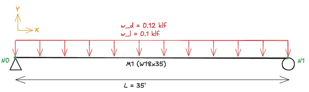
Fig 3. Simply supported beam - example 1.
We can start by importing Pynite’s base class and then instantiating it.
from Pynite import FEModel3D
model = FEModel3D()
3.1 Materials
The next step is adding a material and specifying custom material properties.
# User-defined material
material = "Steel_A992"
E = 29_000  # ksi
nu = 0.3
G = E / (2 * (1 + nu)) # ksi
rho = 0.49 / (12**3)   # kci
Remember, you can use whatever units you prefer. Although imperial units are used here, you can easily swap these out for SI units. The key thing is that you are consistent in your unit selection.
After defining the material, we add it to our model.
# Add material to model
model.add_material(name=material, E=E, G=G, nu=nu, rho=rho)
3.2 Sections
We add a section using the add_section method and pass in the appropriate geometric properties.
# Arbitrarily chosen wide-flange section
model.add_section("W18x35", A=10.3, Iy=15.3, Iz=510, J=0.506)
3.3 Nodes and members
Each node is added individually, and then a member is defined between the nodes.
# Add nodes (35 ft span)
model.add_node('N0', 0, 0, 0)
model.add_node('N1', 35*12, 0, 0)

model.add_member(
    "M1",
    i_node="N0",
    j_node="N1",
    material_name="Steel_A992",
    section_name="W18x35",
    rotation=0,
    tension_only=False,
    comp_only=False
)
3.4 Restraints
Restraints are added by specifying True or False to indicate fixity or not for each degree of freedom.
# Pin support
model.def_support(
    node_name="N0",
    support_DX=True,
    support_DY=True,
    support_DZ=True,
    support_RX=False,
    support_RY=False,
    support_RZ=False
)

# Roller support
model.def_support(
    node_name="N1",
    support_DX=False,
    support_DY=True,
    support_DZ=True,
    support_RX=True,  # For stability
    support_RY=False,
    support_RZ=False
)
3.5 Applied loads
First, we define the magnitudes of the dead and live loads.
# Distributed dead load
w_D = -0.120 / 12  # 0.12 klf to k/in

# Distributed live load
w_L =  -0.100 / 12  # 0.1 klf to k/in
Then, we can apply them to the member, specifying the member name, direction (Fy denoting the local y-axis), start and end position and magnitude as well as a load case assignment.
# Add dead load
model.add_member_dist_load(
    member_name="M1",
    direction="Fy",
    w1=w_D,
    w2=w_D,
    x1=0,
    x2=35*12,  # 35 feet to inches
    case="D"
)

# Add live load
model.add_member_dist_load(
    member_name="M1",
    direction="Fy",
    w1=w_L,
    w2=w_L,
    x1=0,
    x2=35*12,  # 35 feet to inches
    case="L"
)
3.6 Self-weight
I believe there is a minor bug — or at least a source of potential confusion in the add_member_self_weight() method used below. Pynite's documentation clearly distinguishes between global and local coordinate systems, using 'FX', 'FY', and 'FZ' to denote global axes and 'Fx', 'Fy', and 'Fz' for local ones. However, I could not find an explicit convention or explanation for the global coordinate system within the documentation.
Looking at the source code, the add_member_self_weight() method iterates through each member in the model and calculates the self-weight using the expression,
self_weight = factor * member.material.rho * member.section.A
This is applied using add_member_dist_load() with a user-specified global_direction. A more intuitive parameter name might be gravity_direction, with a default factor = -1 to reflect typical gravitational loading.
Moreover, if the method is intended to accept only global directions, it would be clearer and safer to raise an error or warning when a local direction (e.g., 'Fz') is provided. Currently, this distinction isn’t enforced, and no such validation appears to exist.
I’ll reach out to Craig for clarification or perhaps issue a pull request, but for now, let’s note this as a caveat and proceed.
# Add self weight
model.add_member_self_weight(global_direction="FY", factor=-1, case='SW')
3.7 Load combinations
The application of load combinations is pretty self-explanatory. Here, we define the following load combinations:
- D+L
- 1.2D+1.6L
- Dead
- Live
- Self Wt
# Add load combinations
model.add_load_combo(
    name="D+L",
    factors={"SW": 1.0, "D": 1.0, "L": 1.0},
    combo_tags="Service"
)

model.add_load_combo(
    name="1.2D+1.6L",
    factors={"SW": 1.2, "D": 1.2, "L": 1.6},
    combo_tags="Strength"
)

model.add_load_combo(
    name="Dead",
    factors={"SW": 1.0, "D": 1.0},
    combo_tags="Dead"
)

model.add_load_combo(
    name="Live",
    factors={"L": 1},
    combo_tags="Live"
)

model.add_load_combo(
    name="Self Wt",
    factors={"SW": 1},
    combo_tags="Self Weight"
)
3.8 Analysing the model
Now that we have our model and loading fully defined, it’s time to run the analysis. There are 3 types of analyses in Pynite:
-
analyze()- Performs a first-order static analysis and is capable of performing tension/compression-only iterations. -
analyze_linear()- Same asanalyze()but will not consider tension/compression-only elements. -
analyze_PDelta()- Performs a second-order P-Delta analysis.
All of the above analysis methods take axial and bending deformations into account. Shear deformations for beam elements are not implemented.
For our purposes, analyze_linear() will do the trick.
model.analyze_linear(log=True, check_stability=True, check_statics=True)
This returns the following output:
+-------------------+
| Analyzing: Linear |
+-------------------+
- Adding nodal spring support stiffness terms to global stiffness matrix
- Adding spring stiffness terms to global stiffness matrix
- Adding member stiffness terms to global stiffness matrix
- Adding quadrilateral stiffness terms to global stiffness matrix
- Adding plate stiffness terms to global stiffness matrix
- Checking nodal stability

- Analyzing load combination D+L
- Calculating global displacement vector

- Analyzing load combination 1.2D+1.6L
- Calculating global displacement vector

- Analyzing load combination Dead
- Calculating global displacement vector

- Analyzing load combination Live
- Calculating global displacement vector

- Analyzing load combination Self Wt
- Calculating global displacement vector
- Calculating reactions

- Analysis complete

+----------------+
| Statics Check: |
+----------------+

+------------------+--------+--------+--------+--------+--------+--------+--------+---------+--------+---------+-----------+----------+
| Load Combination | Sum FX | Sum RX | Sum FY | Sum RY | Sum FZ | Sum RZ | Sum MX | Sum RMX | Sum MY | Sum RMY |   Sum MZ  | Sum RMZ  |
+------------------+--------+--------+--------+--------+--------+--------+--------+---------+--------+---------+-----------+----------+
|       D+L        |   0    |   0    | -8.93  |  8.93  |   0    |   0    |   0    |    0    |   0    |    0    | -1.87e+03 | 1.87e+03 |
|    1.2D+1.6L     |   0    |   0    | -12.1  |  12.1  |   0    |   0    |   0    |    0    |   0    |    0    | -2.54e+03 | 2.54e+03 |
|       Dead       |   0    |   0    | -5.43  |  5.43  |   0    |   0    |   0    |    0    |   0    |    0    | -1.14e+03 | 1.14e+03 |
|       Live       |   0    |   0    |  -3.5  |  3.5   |   0    |   0    |   0    |    0    |   0    |    0    |    -735   |   735    |
|     Self Wt      |   0    |   0    | -1.23  |  1.23  |   0    |   0    |   0    |    0    |   0    |    0    |    -258   |   258    |
+------------------+--------+--------+--------+--------+--------+--------+--------+---------+--------+---------+-----------+----------+
3.9 Post-processing
Now let’s generate some print statements and results visualisations. We can start with the support reactions.
# Print reactions
print(f"Left Support Reaction: {model.nodes['N0'].RxnFY} kips")
print(f"Right Support Reaction: {model.nodes['N1'].RxnFY} kips")
This gives us the support reactions for each load case defined above.
Left Support Reaction: {'D+L': 4.463350694444444, '1.2D+1.6L': 6.056020833333333, 'Dead': 2.7133506944444443, 'Live': 1.75, 'Self Wt': 0.6133506944444443} kips
Right Support Reaction: {'D+L': 4.463350694444444, '1.2D+1.6L': 6.056020833333333, 'Dead': 2.7133506944444443, 'Live': 1.75, 'Self Wt': 0.6133506944444446} kips
Then, we can move on to the max/min shear and bending moment values.
# Print the max/min shears and moments in the beam
print(f"Maximum Factored Shear: {model.members['M1'].max_shear('Fy', '1.2D+1.6L')} kips")
print(f"Minimum Factored Shear: {model.members['M1'].min_shear('Fy', '1.2D+1.6L')} kip")
print()
print(f"Maximum Factored Moment: {model.members['M1'].max_moment('Mz', '1.2D+1.6L')/12} kip-ft")
print(f"Minimum Factored Moment: {model.members['M1'].min_moment('Mz', '1.2D+1.6L')/12} kip-ft")
print()
print(f"Maximum Moment Dead: {model.members['M1'].max_moment('Mz', 'Dead')/12} kip-ft")
print(f"Minimum Moment Dead: {model.members['M1'].min_moment('Mz', 'Dead')/12} kip-ft")
print()
print(f"Maximum Moment Live: {model.members['M1'].max_moment('Mz', 'Live')/12} kip-ft")
print(f"Minimum Moment Live: {model.members['M1'].min_moment('Mz', 'Live')/12} kip-ft")
print()
This gives us,
Maximum Factored Shear: 6.056020833333333 kips
Minimum Factored Shear: -6.056020833333333 kip

Maximum Factored Moment: 0.0 kip-ft
Minimum Factored Moment: -52.99018229166666 kip-ft

Maximum Moment Dead: 0.0 kip-ft
Minimum Moment Dead: -23.74181857638889 kip-ft

Maximum Moment Live: 1.1842378929335002e-15 kip-ft
Minimum Moment Live: -15.3125 kip-ft
And finally, the deflections.
# Print the max/min deflections in the beam
print(f"Maximum Deflection: {model.members['M1'].max_deflection('dy', 'D+L')} in")
print(f"Minimum Deflection: {model.members['M1'].min_deflection('dy', 'D+L')} in")
Maximum Deflection: 0.0 in
Minimum Deflection: -0.5821786954029269 in
A really nice feature of Pynite is the built-in plotting functionality. This makes it particularly efficient when it comes to generating shear, moment and deflection diagrams.
model.members['M1'].plot_shear(Direction='Fy', combo_name='1.2D+1.6L', n_points=2)
model.members['M1'].plot_moment(Direction='Mz', combo_name='1.2D+1.6L', n_points=50)
model.members['M1'].plot_deflection('dy', combo_name='D+L', n_points=50)
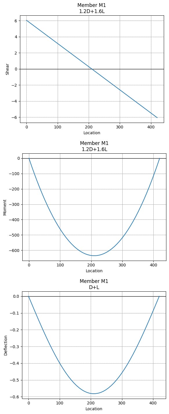
Fig 4. Shear force diagram (top), bending moment diagram (middle), deflection diagram (bottom).
With a basic model under our belt, let’s move on to something a little more involved with our next walkthrough example.
4.0 Example 2 - 2D frame
This example comes from a validation set provided by CSI, and it's one I regularly use to benchmark any new FE software I work with (e.g. fenix, Karamba3D, etc). When using any new analysis tool, it is always a good idea to incorporate a validation step with simple models and hand checks. This will not only give us confidence in using Pynite, but also can help us understand any limitations.
(Spoiler alert: We will see that Pynite's results will exactly match SAP2000's.)
For this example, CSI notes the following:
Only bending deformations are considered in the analysis. Shear and axial deformations are ignored. In SAP2000, this is achieved by setting the property modification factor for area to 1,000 and setting the property modification for shear area to 0.
In this example, we’ll also get our first introduction to Pynite’s impressive rendering capabilities. Consider the 2D frame shown in Fig 5 below.
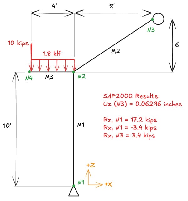
Fig 5. 2D frame structure - example 2.
4.1 Material properties and axial stiffness
We can start by defining the material properties.
material = "Concrete"
E = 3600  # ksi
nu = 0.2
G = E / (2 * (1 + nu))  # ksi
To neglect axial deformations, simply apply an arbitrarily large stiffness modification factor to the area or Young's modulus of the element. Recall that axial stiffness is defined as .
consider_axial_deformation = False
if consider_axial_deformation:
    axial_stiffness_factor = 1
else:
    axial_stiffness_factor = 1000
4.2 Model definition, load assignment and analysis
In example 1, we broke up each step into its own cell for clarity, but in practice, it will be much easier to set up the entire model in one cell.
# Initialise model
frame_model = FEModel3D()

# Add nodes
frame_model.add_node("N1", X=0, Y=0, Z=0)
frame_model.add_node("N2", X=0, Y=0, Z=10*12)
frame_model.add_node("N3", X=8*12, Y=0, Z=16*12)
frame_model.add_node("N4", X=-4*12, Y=0, Z=10*12)

# Add material and section properties
frame_model.add_material(name=material, E=E, G=G, nu=nu, rho=rho)

frame_model.add_section(
    name="12x12",
    A=axial_stiffness_factor*12*12,
    Iy=12**3,
    Iz=12**3,
    J=2.25*(6**4)
)

# Add members
frame_model.add_member(
    name="M1",
    i_node="N1",
    j_node="N2",
    material_name="Concrete",
    section_name="12x12"
)
frame_model.add_member(
    "M2",
    i_node="N2",
    j_node="N3",
    material_name="Concrete",
    section_name="12x12"
)
frame_model.add_member(
    "M3",
    i_node="N4",
    j_node="N2",
    material_name="Concrete",
    section_name="12x12"
)

# Pin support
frame_model.def_support(
    "N1",
    support_DX=True,
    support_DY=True,
    support_DZ=True,
    support_RX=True,  # for stability
    support_RY=False,
    support_RZ=False,
)

# Roller support (free in z-direction)
frame_model.def_support(
    "N3",
    support_DX=True,
    support_DY=False,
    support_DZ=False,
    support_RX=False,
    support_RY=False,
    support_RZ=False,
)

# Add loads
frame_model.add_member_dist_load(
    "M3",
    direction="FZ",
    w1=-1.8 / 12,  # 1.8 klf to k/in
    w2=-1.8 / 12
)
frame_model.add_node_load(
    "N4",
    direction="FZ",
    P=-10,
)

# Run the model!
frame_model.analyze_linear(log=True, check_statics=True)
This gives us the following output.
+-------------------+
| Analyzing: Linear |
+-------------------+
- Adding nodal spring support stiffness terms to global stiffness matrix
- Adding spring stiffness terms to global stiffness matrix
- Adding member stiffness terms to global stiffness matrix
- Adding quadrilateral stiffness terms to global stiffness matrix
- Adding plate stiffness terms to global stiffness matrix
- Checking nodal stability

- Analyzing load combination Combo 1
- Calculating global displacement vector
- Calculating reactions

- Analysis complete

+----------------+
| Statics Check: |
+----------------+

+------------------+--------+-----------+--------+--------+--------+--------+--------+---------+--------+---------+--------+---------+
| Load Combination | Sum FX |   Sum RX  | Sum FY | Sum RY | Sum FZ | Sum RZ | Sum MX | Sum RMX | Sum MY | Sum RMY | Sum MZ | Sum RMZ |
+------------------+--------+-----------+--------+--------+--------+--------+--------+---------+--------+---------+--------+---------+
|     Combo 1      |   0    | -8.82e-13 |   0    |   0    | -17.2  |  17.2  |   0    |    0    |  -653  |   653   |   0    |    0    |
+------------------+--------+-----------+--------+--------+--------+--------+--------+---------+--------+---------+--------+---------+
4.3 Results visualisation
Next, we can print some results.
# Print Results
print(f"Node 3 - Z Deflection: {frame_model.nodes['N3'].DZ} inches")
print(f"Node 1 - Z Reaction: {frame_model.nodes['N1'].RxnFZ} kips")
print(f"Node 1 - X Reaction: {frame_model.nodes['N1'].RxnFX} kips")
print(f"Node 3 - X Reaction: {frame_model.nodes['N3'].RxnFX} kips")
Note that if load combinations are not specified, it will automatically default to "Combo 1". Now let's plot the shear and moment for member "M3".
frame_model.members['M3'].plot_shear(Direction='Fz', n_points=200)
frame_model.members['M3'].plot_moment(Direction='My', n_points=200)
frame_model.members["M3"].plot_deflection(Direction='dz', n_points=20)
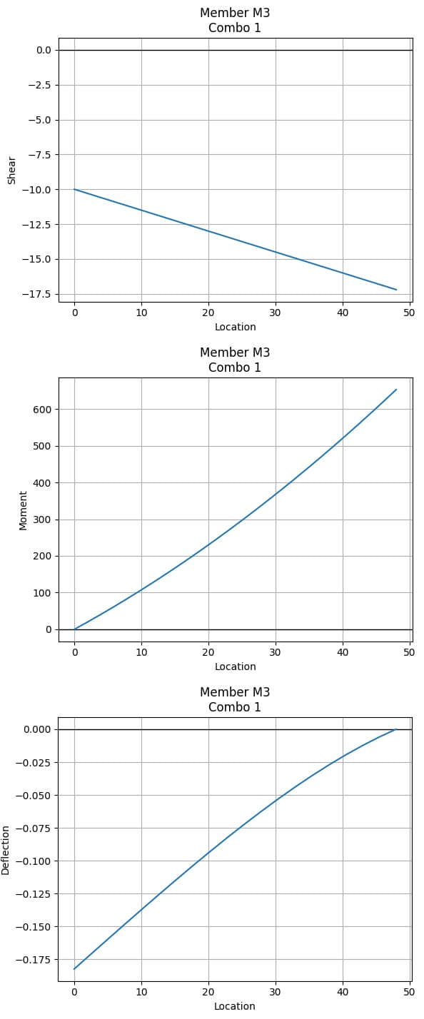
Fig 6. Shear force diagram (top), bending moment diagram (middle), deflection diagram (bottom) for member M3.
4.4 Rendering Pynite models
In a model with multiple members, you can certainly still plot the deflection diagrams for each member (as above). However, it might be more helpful to view the whole model’s deflection using Pynite's Rendering module.
In earlier versions, Pynite used the vtk library for model visualisation. However, this was often clunky and difficult to work with - especially in Jupyter environments. Starting with v0.0.94, Craig introduced a new module, Rendering, which is designed to gradually replace the older Visualization module.
The new Rendering module leverages pyvista, allowing models to be rendered directly within Jupyter notebooks! This results in a much smoother and user-friendly experience.
In this tutorial, we will use Rendering.Renderer(), following Pynite's official recommendation:
Users are urged to switch to using
pyvistarendering instead as VTK rendering is on its way out of Pynite and may be only minimally maintained going forward.
To use the Rendering module, we first need to import it.
from Pynite.Rendering import Renderer
Remember to take a look at Pynite’s documentation on rendering - it contains everything you need to customise your model renders. The rendering process has three simple steps:
- initialise a renderer
- define any render customisations
- call the
render_model()method
Here is a simple implementation with some customisations applied.
rndr = Renderer(frame_model)
rndr.annotation_size = 5
rndr.deformed_shape = True
rndr.deformed_scale = 100
rndr.render_nodes = True
rndr.render_loads = True
rndr.combo_name = 'Combo 1'
rndr.labels = True
rndr.render_model()
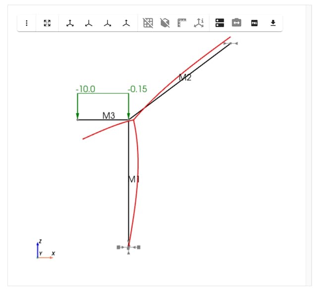
Fig 7. Pynite render of the 2D frame model showing deflection for Combo 1.
Note that we modelled in the X-Z plane (gravity in z-direction), so click the "Reset Camera Y" button in the top row. You can also click and drag around to visualise the model from various angles. The ability to interact with the rendering directly in Jupyter Lab is a very helpful feature!
Rendering in this way does not yet allow us to render the shear force and bending moment diagram for the whole structure. Hopefully, we’ll see this added in a future release.
4.5 Can we do better? Of **kwargs we can! (sorry, I had to..)
Having a boilerplate script that we create once and are able to re-use is a great starting point, but what if we have a structure with hundreds of nodes and elements?
While the main goal of this tutorial is to showcase Pynite and its capabilities, let's take a small side-step to explore how we can more efficiently handle our model data. There are plenty of ways to approach this, but I'll leave you with a simple idea that could be expanded upon: using **kwargs to unpack a dictionary of design data directly into a function call.
Here's the basic concept - you may have noticed in the examples that I've explicitly used keywords when calling methods. This wasn't strictly necessary. For example, the following calls to add_node() are all equivalent:
model.add_node(name="N1", X=0, Y=10, Z=20)
# is the same as...
model.add_node("N1", 0, 10, 20) # <- this is called using "positional" args
# is the same as ..
model.add_node(X=0, name="N1", Z=20, Y=10)
Using keyword arguments makes code more readable and maintainable. It also allows arguments to be passed in any order as long as the names match the function's parameters. Note that when using positional args, the order must map correctly to the method signature!
Now imagine your beam node data is organised like this:
# Note that the keys of the dictionary exactly match the keywords expected in the add_node() method!
nodes = [
{"name": "N1", "X": 0, "Y": 0, "Z": 0},
{"name": "N2", "X": 10, "Y": 20, "Z": 30},
# etc etc
]
By constructing a dictionary for each node's attributes and unpacking with **kwargs, we can dynamically pass arguments to add_node() without hardcoding them. This enables us to scale our function calls effectively. Here is a minimally viable example of how this could be implemented:
# Helper function to add nodes from a dictionary
def add_nodes_from_dict(nodes):
	for node in nodes:
		model.add_node(**node)
In a production setting, you'd want to include error handling (e.g. checking for mismatched list lengths) and eventually wrap this in a proper testing framework.
You might now be asking: how should this data be structured in the first place? Valid question - but that's a topic for another time. It's ultimately a design decision, and there's no single correct answer.
My advice? Start simple and build complexity from there. The simplest form would be a .txt file with node and member definitions. Using Excel as your data source can also be practical - perhaps one sheet for "Nodes", another for "Members", and so on, until all the data needed to build your FEModel3D() is contained in a single Excel file.
You can then use pandas to read the Excel file, iterate through each row, convert it to a dictionary, and dynamically call the relevant functions using **kwargs. Alternatively, csv files could also be used, but multiple files will need to be created for each analogous "Sheet" in Excel.
While I haven't yet integrated this automation step into my own workflows, this is likely how I'd begin if I were to dive in today. To give you a taste, we will utilise dictionary unpacking in Example 3.
5.0 Example 3 - 2D truss (the old reliable)
Many EngineeringSkills readers will have seen this example before - Seán uses this very truss in some of his tutorials and courses. Most recently it served as the test structure for our introduction to OpenSeesPy tutorial (another great alternative to Pynite).
Let's keep the tradition going and analyse this same truss in Pynite! In addition to dictionary unpacking, this example will demonstrate how defining member releases works. Note that this example uses SI units (Newtons and meters).
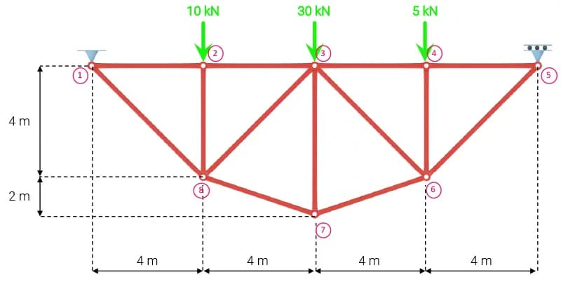
Fig 8. 2D truss structure - example 3.
5.1 Material properties
Again, we start by defining our material properties.
material = "Steel"
E = 200*10**9  #N/m^2
A = 0.005      # m^2
nu = 0.3
G = E / (2 * (1 + nu))  # N/m^2
rho = 7850  # kg/m^3
5.2 Model definition, load assignment and analysis
After initialising our truss model, we define the nodes and elements using the dictionary unpacking strategy we discussed earlier. Even a simple truss example like this emphasises how much cleaner and more scalable this approach to managing model data is.
# Add nodes
nodes = [
    {"name": "N1", "X": 0, "Y": 0, "Z": 0},
    {"name": "N2", "X": 4, "Y": 0, "Z": 0},
    {"name": "N3", "X": 8, "Y": 0, "Z": 0},
    {"name": "N4", "X": 12, "Y": 0, "Z": 0},
    {"name": "N5", "X": 16, "Y": 0, "Z": 0},
    {"name": "N6", "X": 12, "Y": -4, "Z": 0},
    {"name": "N7", "X": 8, "Y": -6, "Z": 0},
    {"name": "N8", "X": 4, "Y": -4, "Z": 0},
]

for node in nodes:
    truss_model.add_node(**node)


# Add material and section properties
truss_model.add_material(name=material, E=E, G=G, nu=nu, rho=rho)

truss_model.add_section(
    name="bar",
    A=A,
    Iy=1, # won't matter because there will be no bending
    Iz=1, # won't matter because there will be no bending
    J=1   # won't matter because there will be no torsion
)

# Add members
members = [
    {"name": "M1", "i_node": "N1", "j_node": "N2", "material_name": "Steel", "section_name": "bar"},
    {"name": "M2", "i_node": "N2", "j_node": "N3", "material_name": "Steel", "section_name": "bar"},
    {"name": "M3", "i_node": "N3", "j_node": "N4", "material_name": "Steel", "section_name": "bar"},
    {"name": "M4", "i_node": "N4", "j_node": "N5", "material_name": "Steel", "section_name": "bar"},
    {"name": "M5", "i_node": "N5", "j_node": "N6", "material_name": "Steel", "section_name": "bar"},
    {"name": "M6", "i_node": "N6", "j_node": "N7", "material_name": "Steel", "section_name": "bar"},
    {"name": "M7", "i_node": "N7", "j_node": "N8", "material_name": "Steel", "section_name": "bar"},
    {"name": "M8", "i_node": "N1", "j_node": "N8", "material_name": "Steel", "section_name": "bar"},
    {"name": "M9", "i_node": "N2", "j_node": "N8", "material_name": "Steel", "section_name": "bar"},
    {"name": "M10", "i_node": "N3", "j_node": "N7", "material_name": "Steel", "section_name": "bar"},
    {"name": "M11", "i_node": "N4", "j_node": "N6", "material_name": "Steel", "section_name": "bar"},
    {"name": "M12", "i_node": "N3", "j_node": "N8", "material_name": "Steel", "section_name": "bar"},
    {"name": "M13", "i_node": "N3", "j_node": "N6", "material_name": "Steel", "section_name": "bar"},
]
for member in members:
    truss_model.add_member(**member)
We simulate axially loaded truss elements by defining appropriate rotational releases at each end of the member.
# Release all member rotations - then go back and fix M1_j, M4_i, and all web members
releases = [
    {"member_name": f"M{i}",
     "Ryi": True,
     "Ryj": True,
     "Rzi": True,
     "Rzj": True}
     for i in range(1, 14)
]
for release in releases:
    truss_model.def_releases(**release)

# Fix internal members and nodes at supports for stability
truss_model.def_releases("M1", Rzj=True)
truss_model.def_releases("M4", Rzi=True)
truss_model.def_releases("M9")
truss_model.def_releases("M10")
truss_model.def_releases("M11")
truss_model.def_releases("M12", Rzi=True, Rzj=True)
truss_model.def_releases("M13", Rzi=True, Rzj=True)
We define nodal point loads and support conditions as seen above and then analyse the complete model.
# Pin support
truss_model.def_support(
    "N1",
    support_DX=True,
    support_DY=True,
    support_DZ=True,
    support_RX=True,  # for stability
    support_RY=False,
    support_RZ=False,
)

# Roller support (free in x-direction)
truss_model.def_support(
    "N5",
    support_DX=False,
    support_DY=True,
    support_DZ=True,
    support_RX=False,
    support_RY=False,
    support_RZ=False,
)

# Add loads
truss_model.add_node_load(
    "N2",
    direction="FY",
    P=-10_000,  # 10 kN downwards
)
truss_model.add_node_load(
    "N3",
    direction="FY",
    P=-30_000,  # 30 kN downwards
)
truss_model.add_node_load(
    "N4",
    direction="FY",
    P=-5_000,  # 5 kN downwards
)

# Run the model!
truss_model.analyze_linear(log=True, check_statics=True)
+-------------------+
| Analyzing: Linear |
+-------------------+
- Adding nodal spring support stiffness terms to global stiffness matrix
- Adding spring stiffness terms to global stiffness matrix
- Adding member stiffness terms to global stiffness matrix
- Adding quadrilateral stiffness terms to global stiffness matrix
- Adding plate stiffness terms to global stiffness matrix
- Checking nodal stability

- Analyzing load combination Combo 1
- Calculating global displacement vector
- Calculating reactions

- Analysis complete

+----------------+
| Statics Check: |
+----------------+

+------------------+--------+-----------+----------+---------+--------+--------+--------+---------+--------+---------+----------+---------+
| Load Combination | Sum FX |   Sum RX  |  Sum FY  |  Sum RY | Sum FZ | Sum RZ | Sum MX | Sum RMX | Sum MY | Sum RMY |  Sum MZ  | Sum RMZ |
+------------------+--------+-----------+----------+---------+--------+--------+--------+---------+--------+---------+----------+---------+
|     Combo 1      |   0    | -2.23e-09 | -4.5e+04 | 4.5e+04 |   0    |   0    |   0    |    0    |   0    |    0    | -3.4e+05 | 3.4e+05 |
+------------------+--------+-----------+----------+---------+--------+--------+--------+---------+--------+---------+----------+---------+
Let’s print the axial forces in the members next.
# Print member axial forces
for member_name, member in truss_model.members.items():
    max_force = member.max_axial()
    print(f"{member_name}: {round(max_force/1000, 2)} kN")
This gives us,
M1: 23.75 kN
M2: 23.75 kN
M3: 21.25 kN
M4: 21.25 kN
M5: -30.05 kN
M6: -27.95 kN
M7: -27.95 kN
M8: -33.59 kN
M9: 10.0 kN
M10: 25.0 kN
M11: 5.0 kN
M12: 1.77 kN
M13: 5.3 kN
As an engineer in the US, I haven't the slightest sense of what these numbers mean (what even is a kilonewton? 🥴). However, it appears that the numbers align with OpenSeesPy!.
For completeness, we’ll also print the nodal displacements.
# Print nodal displacements
for i in range(1, 9):
    node_name = f"N{i}"
    node = truss_model.nodes[node_name]

    dx_value = node.DX.get("Combo 1")
    dy_value = node.DY.get("Combo 1")

    dx_rounded = round(dx_value, 5)
    dy_rounded = round(dy_value, 5)
    print(f"{node_name}: DX= {dx_rounded} m, DY= {dy_rounded} m")
N1: DX= 0.0 m, DY= 0.0 m
N2: DX= -9e-05 m, DY= -0.00063 m
N3: DX= -0.00019 m, DY= -0.00073 m
N4: DX= -0.00027 m, DY= -0.00057 m
N5: DX= -0.00036 m, DY= 0.0 m
N6: DX= -5e-05 m, DY= -0.00055 m
N7: DX= -0.00018 m, DY= -0.00058 m
N8: DX= -0.00032 m, DY= -0.00059 m
And finally, we’ll visualise our complete model and its deflected shape using the Renderer.
rndr = Renderer(truss_model)
rndr.annotation_size = 0.5
rndr.deformed_shape = True
rndr.deformed_scale = 500
rndr.render_nodes = True
rndr.render_loads = True
rndr.combo_name = 'Combo 1'
rndr.labels = True
rndr.render_model()
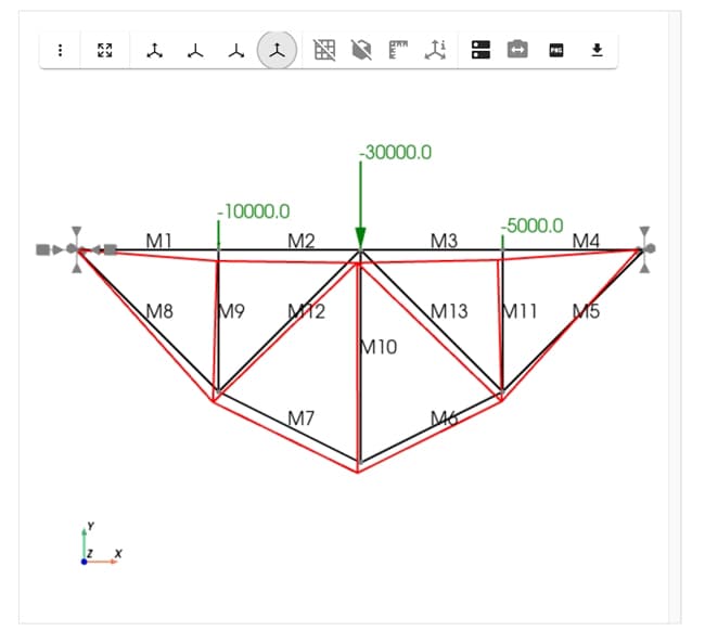
Fig 9. 2D truss model and deflected shape.
In our next example, let's combine another popular open source package, sectionproperties, with Pynite and see how the two can work together.
6.0 Example 4 - Real-world case study
This very simple example is one that was used in the concept phase of a project to quickly iterate on design options (some of the numbers have been altered, but the idea remains unchanged). The client wished to create an opening through a perimeter CMU bearing wall to allow for horizontal expansion of the building, Fig 10.
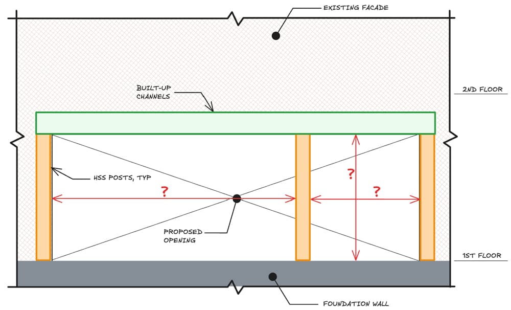
Fig 10. Elevation of proposed opening showing header beam (green) required to carry existing facade.
The idea was to sandwich the existing brick and CMU bearing wall assembly between two built-up channel sections to span the openings, Fig 11.
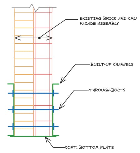
Fig 11. Section through the proposed built-up channel section and wall assembly.
The project made use of sectionproperties to study different channel sizes, then used Pynite to determine the demand and estimate deflections. The demand was then pulled back into sectionproperties for stress analysis, facilitating the design and calculation of the through-bolts.
Since our focus in this tutorial is on getting comfortable with Pynite, we won’t cover stress analysis with sectionproperties here. We’ll actually be digging into that in an upcoming EngineeringSkills tutorial.
To follow along, you'll need to have sectionproperties installed. If you haven't done so already, install it by executing the following command in your terminal:
pip install sectionproperties
If you’re not yet familiar with the sectionproperties library, take a look at my previous tutorial on reinforced concrete column design that made use of both sectionproperties and concreteproperties - a sister-library that focuses on reinforced-concrete section modelling.
Note that sectionproperties defines local coordinates differently than Pynite, so I'll restate their definitions here for clarity:
Pynitelocal coordinate system:- x: along member (torsional axis)
- y: gravity direction (weak axis)
- z: out of plane (strong axis)
sectionpropertieslocal coordinate system:- x: out of plane (strong axis)
- y: gravity direction (weak axis) * z: along member (torsional axis)
6.1 Creating a custom sectionproperties channel
We can import the sectionproperties dependencies as follows:
import sectionproperties.pre.library.steel_sections as steel_geom
from sectionproperties.analysis.section import Section
We’ll start by defining a single channel geometry.
d = 30      # depth, inches
b = 4       # flange width, inches
t_f = 1.75  # flange thickness, inches
t_w = 1.5   # web thickness, inches

channel = steel_geom.channel_section(
    d=d,
    b=b,
    t_f=t_f,
    t_w=t_w,
    r=0,
    n_r=0
)

# View the section
channel
This generates the following image.

Fig 12. Single channel geometry defined using sectionproperties.
Then, we can use the helpful mirror_section() and shift_section() methods to create the double channel geometry.
assembly_width = 12
double_channel = (
    channel.mirror_section(axis='y', mirror_point=(0,0)) +
    channel.shift_section(x_offset=assembly_width)
)

double_channel = double_channel.shift_section(x_offset=-assembly_width/2, y_offset=-d/2)

# View the section
double_channel
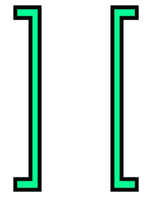
Fig 13. Double channel geometry defined using sectionproperties.
With the geometry defined, we can create a finite element mesh which will allow us to calculate geometric properties.
double_channel.create_mesh(mesh_sizes=0.5)
section = Section(geometry=double_channel)
section.plot_mesh(materials=False)
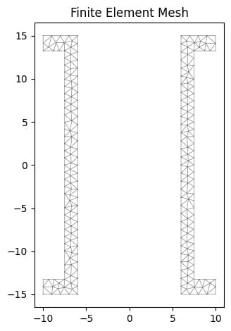
Fig 14. Double channel finite element mesh.
Then we calculate the geometric properties, plot the centroid on the section and display the calculated properties. Note that we have conservatively neglected the stiffening influence of the bottom plate.
section.calculate_geometric_properties()
section.plot_centroids()
section.display_results(fmt=".1f")
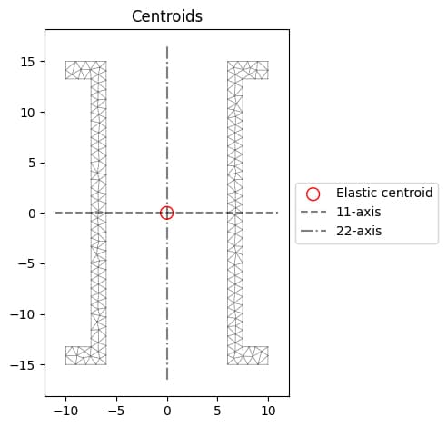
Fig 15. Finite element mesh showing location of centroid calculated using
sectionproperties.
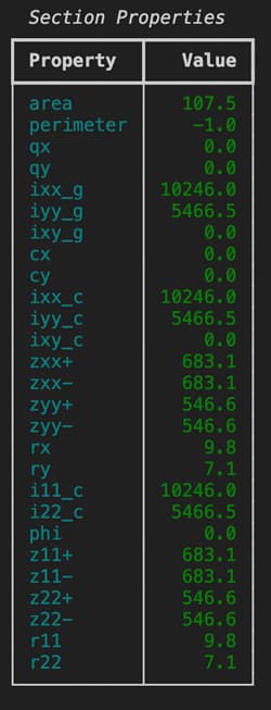
Fig 16. Calculated geometric properties for the double channel section.
We can extract these section properties directly from our section model.
# Note that the sign convention must match Pynite's convention:
# Iz = strong axis, Iy = weak axis, Ix = torsional
Iz, Iy, Ix = section.get_ic()
A = section.get_area()
print(f"{Iz=}, {Iy=}, \n{Ix=}, {A=}")
Iz=10245.989583333336, Iy=5466.458333333332,
Ix=1.072919530997751e-12, A=107.50000000000001
Now that we have our trial section properties, we can apply them in a Pynite model.
6.2 Pynite model definition
The definition of our Pynite model and the associated loading all proceed as normal - the only thing to note is that we’re assigning cross-section properties within our Pynite model that have been calculated based on our custom sectionproperties model.
# Define material properties
E = 29_000  # ksi
nu = 0.3
G = E / (2 * (1 + nu))  # ksi
rho = 0.49 / (12**3)  # kci

x_1 = 37 * 12  # inches
x_2 = 52 * 12  # inches

beam_model = FEModel3D()

beam_model.add_material("Steel", E, G, nu, rho)

beam_model.add_node("N1", X=0, Y=0, Z=0)
beam_model.add_node("N2", X=x_1, Y=0, Z=0)
beam_model.add_node("N3", X=x_2, Y=0, Z=0)

beam_model.add_section(
    name="Double Channel",
    A=A,
    Iy=Iy,
    Iz=Iz,
    J=0  # irrelevant to this analysis
)

beam_model.add_member(
    name="M1",
    i_node="N1",
    j_node="N3",
    material_name="Steel",
    section_name="Double Channel"
)

# Pin
beam_model.def_support(
    "N1",
    support_DX=True,
    support_DY=True,
    support_DZ=True,
    support_RX=True,  # for stability
    support_RY=False,
    support_RZ=False
)

# Rollers
beam_model.def_support(
    "N2",
    support_DX=False,
    support_DY=True,
    support_DZ=True,
    support_RX=True,
    support_RY=False,
    support_RZ=False
)
beam_model.def_support(
    "N3",
    support_DX=False,
    support_DY=True,
    support_DZ=True,
    support_RX=True,
    support_RY=False,
    support_RZ=False
)

# Add self weight of double channel
beam_model.add_member_self_weight(global_direction="FZ", factor=-1, case='SW')

wall_weight = -4 / 12  # 4 klf to k/in

# Add dead load
beam_model.add_member_dist_load(
    member_name="M1",
    direction="FZ",
    w1=wall_weight,
    w2=wall_weight,
    x1=0,
    x2=x_2,
    case="D"
)

beam_model.add_load_combo(name="1.0D", factors={"SW": 1, "D": 1})
beam_model.add_load_combo(name="1.4D", factors={"SW": 1.4, "D": 1.4})

beam_model.analyze(check_statics=True)
6.3 Pynite results visualisation
Our results visualisation also proceeds as per the previous examples. We plot the shear and moment diagrams and the deflected shape for a specific load case, print some max/min results and finish up with a render of the structure and deflected shape.
beam_model.members['M1'].plot_shear(Direction="Fz", combo_name="1.4D", n_points=20)
beam_model.members['M1'].plot_moment(Direction="My", combo_name="1.4D", n_points=200)
beam_model.members['M1'].plot_deflection("dz", combo_name="1.0D", n_points=200)
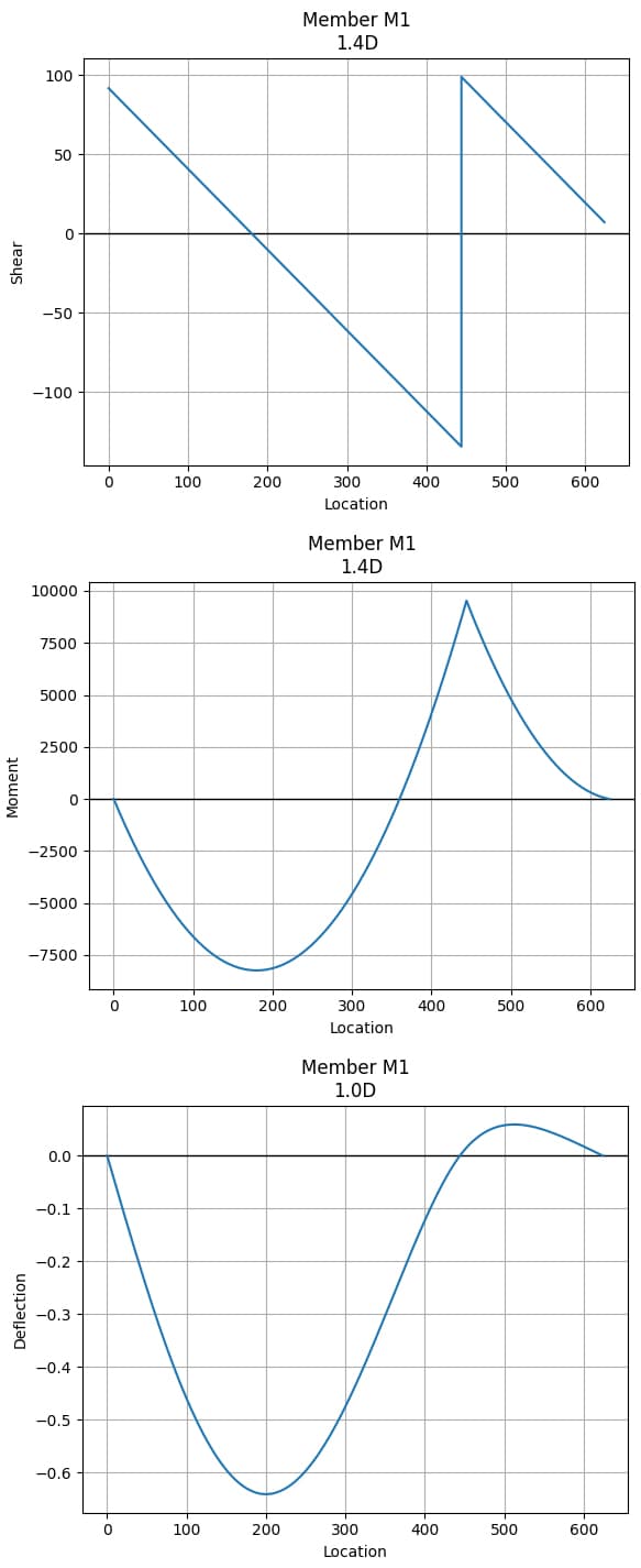
Fig 17. Shear force diagram (top), bending moment diagram (middle), deflection diagram (bottom) double channel beam.
# Print reactions
print(f"Left Support Reaction: {beam_model.nodes['N1'].RxnFZ} kips")
print(f"Middle Support Reaction: {beam_model.nodes['N2'].RxnFZ} kips")
print(f"Right Support Reaction: {beam_model.nodes['N3'].RxnFZ} kips")

# Print the max/min shears and moments in the beam
print(f"Maximum Factored Shear: {beam_model.members['M1'].max_shear('Fz', '1.4D')} kips")
print(f"Minimum Factored Shear: {beam_model.members['M1'].min_shear('Fz', '1.4D')} kip")
print(f"Maximum Factored Moment: {beam_model.members['M1'].max_moment('My', '1.4D')/12} kip-ft")
print(f"Minimum Factored Moment: {beam_model.members['M1'].min_moment('My', '1.4D')/12} kip-ft")
print(f"Maximum Moment Dead: {beam_model.members['M1'].max_moment('My', '1.0D')/12} kip-ft")
print(f"Minimum Moment Dead: {beam_model.members['M1'].min_moment('My', '1.0D')/12} kip-ft")

# Print the max/min deflections in the beam
print(f"Maximum Deflection: {beam_model.members['M1'].max_deflection('dz', '1.0D')} in")
print(f"Minimum Deflection: {beam_model.members['M1'].min_deflection('dz', '1.0D')} in")
Left Support Reaction: {'1.0D': 65.44273120777028, '1.4D': 91.61982369087836} kips
Middle Support Reaction: {'1.0D': 166.63584662787787, '1.4D': 233.290185279029} kips
Right Support Reaction: {'1.0D': -5.057050057870377, '1.4D': -7.0798700810185125} kips

Maximum Factored Shear: 98.76164091435183 kips
Minimum Factored Shear: -134.52854436467715 kip

Maximum Factored Moment: 793.811332465278 kip-ft
Minimum Factored Moment: -686.6843880345054 kip-ft

Maximum Moment Dead: 567.0080946180557 kip-ft
Minimum Moment Dead: -490.4888485960757 kip-ft

Maximum Deflection: 0.05923470093565157 in
Minimum Deflection: -0.6412486371012381 in
rndr = Renderer(beam_model)
rndr.annotation_size = 15
rndr.deformed_shape = True
rndr.deformed_scale = 100
rndr.render_nodes = True
rndr.render_loads = True
rndr.combo_name = '1.4D'
rndr.labels = True
rndr.render_model()
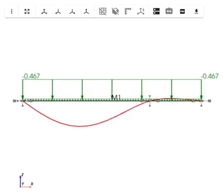
Fig 18. Render of the complete structural model showing the scaled deflected shape.
Now that we’ve identified the maximum shear, moment, and deflection, we can tweak the model as needed to satisfy both strength and serviceability requirements. In this particular case, deflection governed the design to mitigate cracking in the existing brick facade.
Having a quick, lightweight analysis strategy for a condition like this made it easy to iterate through design options during the schematic phase. It also gave the client real-time feedback on how their decisions could affect the structure and incorporate input from the general contractor.
Some of the key questions that came up during this process included:
-
What happens if we relocate the middle post?
-
How does increasing the height of the opening affect the design?
-
Can we reduce the flange width and still meet performance criteria?
Hopefully by now, you can see how these kinds of questions are easily explored using the small script we’ve developed.
7.0 Conclusion
Open source libraries like Pynite give structural engineers an opportunity to step outside the confines of commercial software to quickly analyse simple systems. They're not just for hobbyists or programmers - they're practical, accessible, and increasingly essential in a modern engineer's workflow. By learning to work with tools like Pynite, you can validate results, explore different design options quickly, or automate repetitive tasks.
The part 2 of this series, we cover the analysis of plate structures using Pynite. You can read that and download the accompanying code here.
All Access Membership
Learn, revise or refresh your knowledge and master engineering analysis and design

Access Every Course and Tool
- Over 1140 lectures & over 234 hours of HD video content
- Access member-only 'deep dive' tutorials
- Access all downloads, pdf guides & Python codes
- Access to the StructureWorks Blender addon + updates
- Packed development roadmap of courses & tutorials
- Price Guarantee – avoid future price rises as we grow
- Priority Q&A support
- Course completion certificates
- Early access to new courses
Featured Tutorials and Guides
If you found this tutorial helpful, you might enjoy some of these other tutorials.

Beam Design using the American Institute of Steel Construction (AISC) Manual
A US-centric deep dive into the design of code-compliant steel beams

Dan Ki

A primer on the form and behaviour of gridshell structures
The evolution of gridshells and techniques for form finding and analysis

Dr Seán Carroll
