An Introduction to Uniform Torsion in Cylindrical Shafts

The Fundamental Engineering Mechanics Series – Part 3

Welcome to part 3 of the Fundamental Engineering Mechanics tutorial series. This part will focus on torsion in circular shafts and the stresses and strains it induces. For the previous instalment in the series, go here.

In the previous tutorial in this series, we covered free-body diagrams and how to calculate reaction forces. It may seem like quite a jump to now be exploring torison in part 3. This is because, before torsion, I would usually suggest covering truss analysis and shear force and bending moment analysis for beams and frames. But I’ve already covered these in multiple tutorials, so there’s no need to cover them again as part of this series. Feel free to cover those before diving into Torsion with me here.

1.0 Introducing torsion

As mentioned above, in previous tutorials, we’ve discussed trusses and observed that the members that make up a truss experience only axial force. We could say that the action experienced by these members is axial force. We’ve also discussed structural elements whose primary actions were shear forces and bending moments (beams and frames).

We should clarify here that what distinguishes an axial force from a shear force is simply the axis along which the force is applied. Axial forces have their line of action parallel to the longitudinal axis of the member, while shear forces have a line of action perpendicular to this axis.

When discussing bending moments applied to 2D structures in the x-y plane, we didn’t labour the point at the time, but the moments considered were all about an axis perpendicular to the x-y plane (page or screen) – the z-axis, see Fig 1 below.

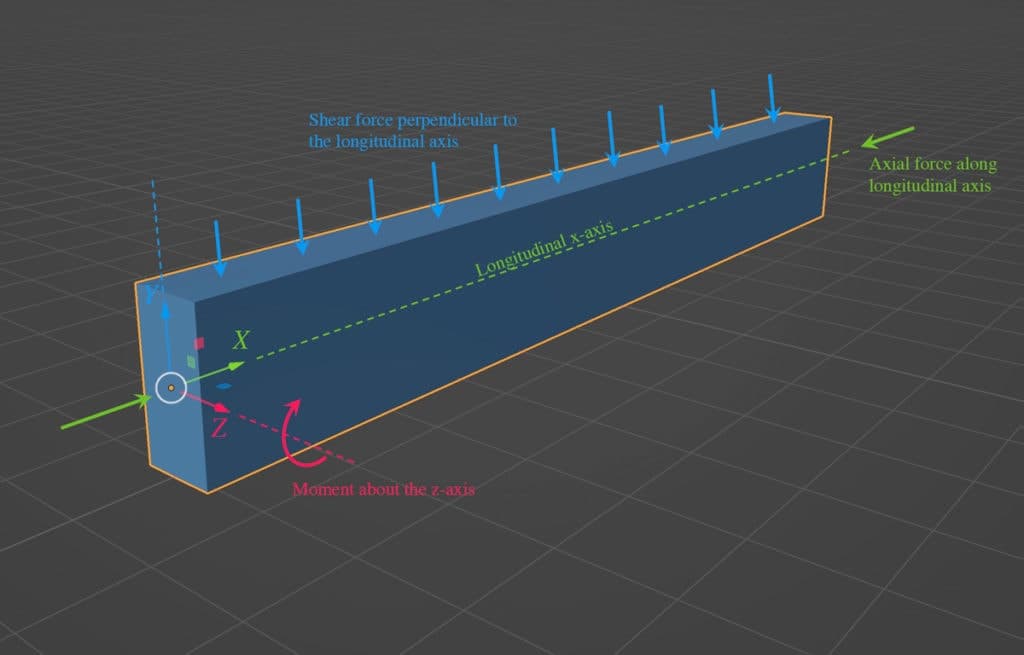
Intro to torsion 1 | EngineeringSkills.com

Fig 1. Beam subject to shearing forces (blue), axial force (green) and bending moment (pink). All of these actions have been discussed in previous tutorials.

In this tutorial, we introduce another action – torsion. This is simply a bending moment applied about a different axis – the longitudinal axis, Fig 2. Torsion will cause twisting about the longitudinal axis and is a very common form of loading that we need to be able to analyse. We often refer to torsional moments as torques (we can use the terms torsional moment and torque interchangeably).

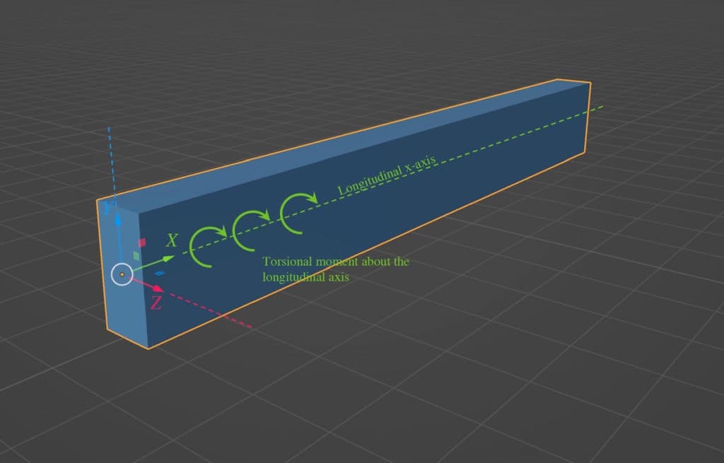
Intro to torsion 2 | EngineeringSkills.com

Fig 2. Beam subject to a torsional moment about the longitudinal x-axis.

We can represent torsion (or any moment) with the curved arrow you’ll be familiar with from previous tutorials or with a double-headed straight arrow. The double-headed arrow is typically more convenient for representing torsion applied to 2D structures. To determine the sense of rotation indicated by a double-headed arrow, we use the right hand screw rule.

According to this sign convention, if you point the thumb or your right hand in the direction of the double-headed arrow and make a fist, your fingers will curve around and point in the direction of the positive sense of rotation for the torque. This will be an important convention to understand and keep in mind.

2.0 Torsional Deformation

Our starting point here will be to explore the concept of strain as it applies to circular bars and to derive an equation that relates the strain to the angle of twist in the bar. First, let’s state some assumptions that will apply to our discussion:

the bar or shaft is circular in cross-section and prismatic, which means it has the same cross-section shape throughout its length.
the angle of twist between both ends of the bar, which we’ll denote as $\phi$ , remains small.
the applied torque is constant throughout the length of the bar – we therefore refer to the bar as being in pure torsion.
angles of twist are measured in radians, recall that $\pi\: \text{radians}=180^\circ$ .

Consider the bar with cross-sectional radius $r$ and length $L$ , pictured below. It’s fixed against torsional rotation at end $p$ . The applied torque at $q$ , $T$ , induces an angle of twist $\phi$ such that point $q$ rotates around to point $q'$ at the free end of the bar. We also note that the angle of twist varies linearly between $x=0$ and $x=L$ .

Intro to torsion 3 | EngineeringSkills.com

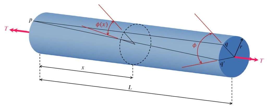
Fig 3. Prismatic circular bar subject to torque $T$ , showing resulting angular deformation $\phi(x)$

Like all good engineering derivations, we now consider a small segment of the bar with length $\mathrm{d}x$ , pictured below. We note that the right cross-section rotates relative to the left cross-section by an amount $\mathrm{d}\phi$ . As a result, the original element $abcd$ becomes $ab'c'd$ with $b$ rotating to $b'$ and $c$ rotating to $c'$ .

Because we’ve made the initial assumption that the angle of rotation between the ends of the bar is small, we can say that the lengths of the sides $ab'$ and $dc'$ remain unchanged. From this, we can conclude that the deformation of the element $abcd$ is completely defined by the decrease in the angle $\angle bad$ . We recognise this as a shear deformation, $\gamma$ , and conclude that the element is in pure shear which means it is only experiencing shear strain, as opposed to normal strains that would be induced by axial forces or bending moments.

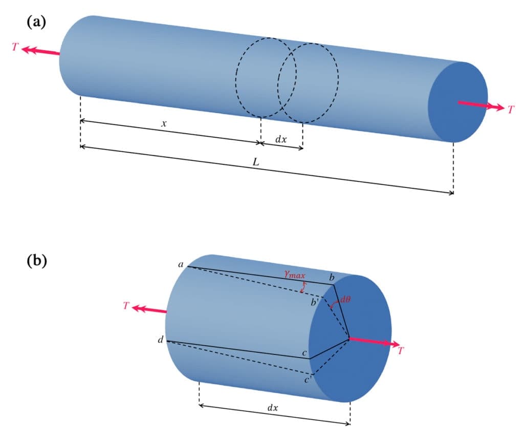
Intro to torsion 4 | EngineeringSkills.com

Fig 4. (a) Prismatic circular bar in a state of pure torsion. (b) Sub-length $\mathrm{d}x$ experiencing an angle of twist $\mathrm{d}\phi$ giving rise to a shear deformation $\gamma_{\text{max}}$ on the outer surface of the bar.

We can see from Fig 4(a) above that the magnitude of the shear strain $\gamma_{\text{max}}$ is given by,

\gamma_{\text{max}} = \frac{bb'}{\mathrm{d}x} \tag{1}

We note that for small angles we can replace the distance $bb'$ with $r\:\mathrm{d}\phi$ , yielding,

\gamma_{\text{max}} = \frac{r\:\mathrm{d}\phi}{\mathrm{d}x} \tag{2}

The quantity $\mathrm{d}\phi/\mathrm{d}x$ is the rate of twist or twist per unit length and is replaced by $\theta$ ,

\theta = \frac{\mathrm{d}\phi}{\mathrm{d}x} \tag{3}

As a result, we obtain the equation for the shear strain at radius $r$ ,

\boxed{\gamma_{\text{max}} = r\theta} \tag{4}

Note that for elements of length $L$ experiencing pure torsion (constant torque magnitude throughout the bar), $\theta = \phi/L$ and for pure torsion only we have,

\boxed{\gamma_{\text{max}} = \frac{r\phi}{L}} \tag{5}

We can see from the preceding equations that for any given cross-section the shear strain varies linearly with the radius. For hollow circular tubes, for example, we can obtain the shear strain magnitude at the inner and outer walls simply by substituting the relevant value for the radius, (see below). Therefore, the max in the subscript $\gamma_{\text{max}}$ refers to the fact that this shear strain was evaluated for the outer surface of the bar, where the radius and therefore shear strain are a maximum.

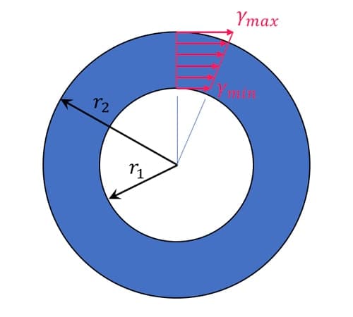
Fig 5. Shear strain $\gamma$ varies linearly with radius.

3.0 Torsion in linearly elastic circular bars

So, at this point, we have an equation that relates the angle of twist with the associated shear strain. Next, we’d like to tie this into the shear stress, $\tau$ . If the bar is made of a linearly elastic material, we know the shear stress will be linearly proportional to the shear strain. In the case of shear (as opposed to tension and compression), the stress $(\tau)$ and strain $(\gamma)$ are related by the shear modulus of elasticity, $G$ ,

\tau = G\gamma \tag{6}

We can therefore state the shear stress, $\tau$ at a radius $r$ as,

\boxed{\tau = G r \theta} \tag{7}

If we wish to determine the shear stress at some internal radius $\rho$ , we could do so as follows,

\tau = \frac{\rho}{r}\tau_{\text{max}} \tag{8}

where $\tau_{\text{max}}$ is the maximum shear stress on the outer surface.

Figure 6(a) below shows a bar in pure torsion and an enlarged stress element with the directions of the resulting shear stresses at the surface indicated. In image (b), we can see the shear stresses and corresponding shear deformation on the element. We again see in image (c) that the shear stress varies linearly with radius.

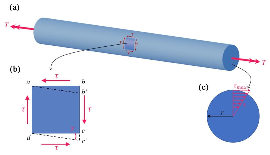
Intro to torsion 6 | EngineeringSkills.com

Fig 6. (a) Bar in pure torsion, (b) resulting stresses and strains reflected on an element taken from the bar, (c) cross-section of the bar showing linear variation of shear stress with radius.

3.1 Relating shear stress with torque

Now we’ll derive the torsion formula that relates the applied torque $T$ with the shear stress induced, $\tau$ . We start by considering the stressed cross-section and an element of area within this cross-section $\mathrm{d}A$ (see Fig 7 below). This infinitesimal area is located at radius $\rho$ and experiences a shear stress, $\tau$ . Therefore we can calculate the force experienced by $\mathrm{d}A$ as $\tau \mathrm{d}A$ . This force generates a moment about the axis of the bar, $\mathrm{d}M$ .

\mathrm{d}M = \tau \rho \mathrm{d}A \tag{9}

Replacing $\tau$ with the expression we derived previously yields,

\mathrm{d}M = \frac{\tau_{\text{max}}}{r} \rho^2 \mathrm{d}A \tag{10}

Note that the summation of all of the moments $\mathrm{d}M$ , acting on all elements of area $\mathrm{d}A$ , equals the applied torque, $T$ . We can perform this summation by integrating $\mathrm{d}M$ over the full cross-sectional area,

T = \int_A \mathrm{d}M = \frac{\tau_{\text{max}}}{r}\int_A \rho^2 \mathrm{d}A \tag{11}

We now define the polar moment of inertia of the circular cross-section, $I_P$ ,

I_P = \int_A \rho^2 \mathrm{d}A \tag{12}

This is a property of the cross-section shape (analogous to the second moment of area, $I$ , which we encounter when considering flexural rigidity, $EI$ in bending). For a circle with diameter $d$ , the polar moment of inertia is given by,

I_P = \frac{\pi d^4}{32} \tag{13}

Therefore we have,

T = \frac{\tau_{\text{max}}}{r}I_P \tag{14}

Rearranging, we obtain the torsion formula,

\boxed{\tau_{\text{max}} = \frac{T r}{I_p}} \tag{15}

Intro to torsion 7 | EngineeringSkills.com

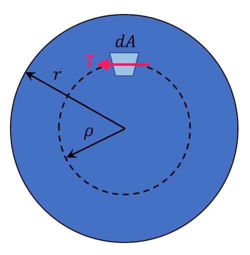
Fig 7. Cross-section of a bar in pure torsion showing an element of area $\mathrm{d}A$ experiencing a torsional stress $\tau$ .

If we recall our expression from above, $\tau_{\text{max}} = Gr\theta$ where $\theta$ was the rate of twist or twist per unit length, we can combine this with the torsion formula to obtain,

\theta = \frac{T}{GI_P} \tag{16}

In the above equation, the quantity $GI_P$ is known as the torsional rigidity and is analogous to the flexural rigidity $EI$ for bending.

Limitations

Our discussion and derivations so far have assumed the material remains linearly elastic and at no time is the applied torque such that the proportional limit for the material is exceeded. Our derivations are also only valid in the absence of stress concentrations that result from discontinuities in geometry or at points of load application. Next, we can consider some numerical examples to demonstrate these equations in action.

3.2 Example 1

Consider a solid steel bar with a circular cross-section. The bar is subject to an applied torque $T=800\:Nm$ and has the following parameter values:

diameter $d = 50\:mm$
length $L=2.0\:m$
shear modulus $G = 75\:kN/mm^2$

Use this information to:

Determine the maximum shear stress that develops in the bar
Determine the angle of twist between the bar ends
If the maximum allowable shear stress is $35 \:N/mm^2$ and the maximum allowable angle of twist is $1.75^\circ$ , what is the maximum allowable torque?

Solution

(1) The maximum shear stress is obtained using,

\tau_{\text{max}} = \frac{T r}{I_p}

We’ll use some simple Python to perform the calculations but you can easily work this out with a pen and paper if you prefer.

import math #Basic math functionality
import numpy as np #Numpy for working with arrays
G = 75*10**9 #(N/m^2)
L = 2 #(m)
T = 800 #(Nm)
d = 0.05 #(m)
r = d/2 #(m)
Ip = math.pi*d**4/32 #(m^4)
tau_max = T*r/Ip #(N/m^2)
print(f'The maximum shear stress is {round(tau_max/10**6,1)} N/mm^2')

-> The maximum shear stress is 32.6 N/mm^2

(2) The angle of twist is obtained using,

\phi = \frac{TL}{GI_P}

phi_radians = T*L/(G*Ip) #(rads)
phi_deg = phi_radians*180/math.pi #(deg)
print(f'The angle of twist between ends is {round(phi_radians,3)} radians or {round(phi_deg,2)} degrees')

-> The angle of twist between ends is 0.035 radians or 1.99 degrees

(3) Let’s first assume the torque is limited by the maximum allowable shear stress, $\tau_{\text{max}}=35\:N/mm^2$ . In this case, we can solve for the maximum torque by rearranging the torsion formula as follows,

T = \frac{\tau_{\text{max}}I_p}{r}

tau_max = 35 #(N/mm^2)
T_max_1 = (tau_max*10**6)*Ip/r
print(f'The maximum torque limited by shear stress is {round(T_max_1,1)} Nm')

-> The maximum torque limited by shear stress is 859.0 Nm

Now we can test what the maximum torque would be if the angle of twist were the limiting criteria using,

T = \frac{\phi G I_p}{L}

phi_max_deg = 1.75 #(degrees)
phi_max_rad = phi_max_deg*math.pi/180 #(rads)
T_max_2 = phi_max_rad*G*Ip/L
print(f'- The maximum torque limited by angle of twist is {round(T_max_2,1)} Nm')

-> The maximum torque limited by angle of twist is 702.8 Nm

We can see that the maximum allowable torque is $702.8\:Nm$ and is limited by the allowable angle of twist specified. However, keeping with the Python theme here and so that we have a reusable code that yields the final answer without our intervention at the end, we’ll write some code to output the final conclusion.

#Programmatically test which is the limiting factor
if(T_max_1<T_max_2):
  print(f'(c) The maximum allowable torque is {round(T_max_1,1)} Nm, limited by shear stress')
elif(T_max_1>T_max_2):
  print(f'(c) The maximum allowable torque is {round(T_max_2,1)} Nm, limited by angle of twist')
else:
  print(f'(c) The allowable torque is {round(T_max_1,1)} Nm and simultaneously limited by shear stress and angle of twist')

-> The maximum allowable torque is 702.8 Nm, limited by angle of twist

3.3 Example 2

Consider two shafts, one hollow and one solid. Both have an outer diameter $D$ while the hollow shaft has an inner diameter of $0.75D$ . Both shafts experience a torque $T$ . Our task is to analyse the relative efficiency of each shaft at transmitting torque. We’ll do this by establishing the ratio of the following properties for each shaft:

shear stress
angle of twist
weight

Solution

(a) If the torque and outer radius are the same, the shear stress is proportional to $1/I_P$ . Therefore we simply need to compare the ratio of $I_P$ values to obtain a ratio for shear stress for the shafts. For the solid shaft,

I_P = \frac{\pi D^4}{2}

For the hollow shaft,

I_P = \frac{\pi D^4}{2} - \frac{\pi (0.75D)^4}{2}

D_outer = 1 #Value representing outer diameter
D_ratio = 0.75 #Ratio of diameters, D_inner/D_outer
Ip_solid = (math.pi*D_outer**4)/2
Ip_hollow = Ip_solid - (math.pi*(D_ratio*D_outer)**4)/2

tau_ratio = (1/Ip_hollow)/(1/Ip_solid)
print(f'(a) The ratio of maximum shear stress in the hollow shaft to that on the solid shaft is {round(tau_ratio,2)}')
print(f'In other words the hollow shaft experiences a {round(100*(tau_ratio-1))}% larger maximum stress for the same applied torque')

-> (a) The ratio of maximum shear stress in the hollow shaft to that on the solid shaft is 1.46
-> (b) In other words the hollow shaft experiences a 46% larger maximum stress for the same applied torque

(b) Because both shafts are the same length and made of the same material, the angles of twist are also proportional to the inverse of the polar moment of inertia, therefore…

print(f'(b) The ratio of angle of twist in the hollow shaft to that on the solid shaft is also {round(tau_ratio,2)}')
print(f'Again, the hollow shaft experiences {round(100*(tau_ratio-1))}% more rotation for the same applied torque')

-> (b) The ratio of angle of twist in the hollow shaft to that on the solid shaft is also 1.46
-> Again, the hollow shaft experiences 46% more rotation for the same applied torque

A_solid = math.pi*D_outer**2
A_hollow = A_solid - math.pi*(D_ratio*D_outer)**2
weight_ratio = A_hollow/A_solid
print(f'(c) The ratio of weight of the hollow shaft to that of the solid shaft is {weight_ratio}')
print(f'The hollow shaft is {round(100*(1-weight_ratio))}% lighter than the equivalent diameter solid shaft')

-> (c) The ratio of weight of the hollow shaft to that of the solid shaft is 0.4375
-> The hollow shaft is 56% lighter than the equivalent diameter solid shaft

From this analysis, we can see the inherent efficiency offered by a hollow shaft. Although it develops a larger magnitude shear stress under the same applied torque and a larger rotation, it is significantly lighter. So, if the material the shaft is made from can withstand the larger stress and if the larger angle of twist can be accommodated, it makes more sense to select a hollow shaft.

We can get a better sense of how these relationships change by plotting the ratios for different values of diameter ratio. Since we’ve already written the code to perform the calculation for one diameter ratio, all we need to do is wrap this in a for loop and save the values calculated on each iteration.

#Outer diameter values are constant
D_outer = 1
Ip_solid = (math.pi*D_outer**4)/2
A_solid = math.pi*D_outer**2

#Containers to hold our calculated ratios
tr = np.array([])
wr = np.array([])
R = np.arange(0.1,0.81,0.01) #A selection of diameter ratios
for r in R:
  D_ratio = r #Ratio of diamters, D_inner/D_outer
  Ip_hollow = Ip_solid - (math.pi*(D_ratio*D_outer)**4)/2
  A_hollow = A_solid - math.pi*(D_ratio*D_outer)**2

  tau_ratio = (1/Ip_hollow)/(1/Ip_solid) #Shear stress ratio
  tr = np.append(tr, tau_ratio) #Save for later

  weight_ratio = A_hollow/A_solid #Weight ratio
  wr = np.append(wr, weight_ratio) #Save for later

Now that we have all of the values calculated and saved, we can plot them so see the behaviour more clearly.

import matplotlib.pyplot as plt #Plotting functionality

fig, ax1 = plt.subplots(figsize=(12,6))
ax2 = ax1.twinx()
ax1.plot(R,tr,'b')
ax2.plot(R,wr,'r')

#Housekeeping
ax1.set_xlabel('Diameter ratio (Di/Do)')
ax1.set_ylabel('Stress ratio', color='b')
ax2.set_ylabel('Weight ratio',color='r')
ax1.set_title('Diameter ratio versus stress and weight ratios')
ax1.set_xlim([0.1,1])plt.grid()plt.show()

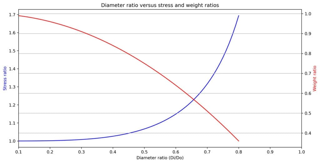
Intro to torsion 8 | EngineeringSkills.com

Fig 8. Plot of stress ratio and weight ratio against ratio of inner and outer shaft diameters.

The blue line shows us how the hollow tube generates more stress when compared to the solid tube, as the inner diameter approaches the outer diameter and the walls of the tube get thinner. At the same time, we can see from the red line how the weight of the hollow tube progressively reduces. Note that the cross-over point here does not have any special significance as we have two different y-scales.

3.4 Example 3

A circular steel shaft must transmit a torque of $5000\:Nm$ without exceeding an allowable shear stress of $50\:N/mm^2$ or an allowable rate of twist of $0.45^\circ/m$ . The shear modulus of elasticity is $75\: GPa$ . A hollow or solid shaft may be used. To assess the suitability of each option:

determine the required diameter of the solid shaft, $d$
determine the required outer diameter of the hollow shaft, $d_o$ , if the wall thickness is $10\%$ of the outer diameter
determine the diameter ratio between shafts, $d_o/d$ and the ratio of weights of the hollow and solid shafts

Solution

For the solid and hollow shaft, the diameter may be limited by either the allowable shear stress or allowable rate of twist. We need to determine diameters based on both criteria and select the largest as the minimum diameter for each shaft. To evaluate a diameter limited by the allowable stress we will use,

\tau_{\text{max}} = \frac{T r}{I_p}

To evaluate a diameter limited by the allowable rate of twist we will use,

\theta = \frac{T}{GI_p} \tag{17}

In both cases, we can rearrange and solve to determine the diameter.

#CONSTANTS
T = 5000 #(Nm)
tau_max = 50*10**6 #(N/m^2)
theta_max = 0.45 #(deg/m)
theta_max_rad = theta_max*math.pi/180 #(rads)
G = 75*10**9 #(N/m^2)

#SOLID SHAFT - LIMITED BY ALLOWABLE SHEAR STRESS
r = ((2*T)/(math.pi*tau_max))**(1/3)
d_solid_1 = 2*r #(m) Solid diameter limited by shear stress

#SOLID SHAFT - LIMITED BY ALLOWABLE RATE OF TWIST
r = ((2*T)/(math.pi*G*theta_max_rad))**(1/4)
d_solid_2 = 2*r #(m) Solid diameter limited by rate of twist

#Determine which condition governs
if(d_solid_1>d_solid_2):
  d_solid = d_solid_1
  print(f'(a). The req. dia. of the solid shaft is {round(d_solid_1,3)} m, limited by allowable shear stress')
elif(d_solid_1<d_solid_2):
  d_solid = d_solid_2
  print(f'(a). The req. dia. of the solid shaft is {round(d_solid_2,3)} m, limited by allowable rate of twist')
else:
  d_solid = d_solid_1
  print(f'(a). The req. dia. of the solid shaft is {round(d_solid_1,3)} m, simultaneously limited by allowable shear stress and rate of twist')

-> (a). The req. dia. of the solid shaft is 0.096 m, limited by allowable rate of twist

For the hollow shaft we note the inner diameter, $d_i = 0.8\times d_o$ . Therefore,

\begin{align*} I_P &= \frac{\pi}{32}\left(d_o^4 - (0.8d_o)^4\right)\\ I_P &= \frac{\pi}{32}\left(0.5904 \:d_o^4\right)\\ I_P &= 0.058\:d_o^4 \end{align*}

#HOLLOW SHAFT - LIMITED BY ALLOWABLE SHEAR STRESS
d_hollow_1 = ((0.5*T)/(0.058*tau_max))**(1/3) #(m) Hollow outer diameter limited by shear stress

#HOLLOW SHAFT - LIMITED BY ALLOWABLE RATE OF TWIST
d_hollow_2 = (T/(G*theta_max_rad*0.058))**(1/4)

#Determine which condition governs
if(d_hollow_1>d_hollow_2):
  d_hollow = d_hollow_1
  print(f'(b). The req. outer dia. of the hollow shaft is {round(d_hollow_1,3)} m, limited by allowable shear stress')
elif(d_solid_1<d_solid_2):
  d_hollow = d_hollow_2
  print(f'(b). The req. outer dia. of the hollow shaft is {round(d_hollow_2,3)} m, limited by allowable rate of twist')
else:
  d_hollow = d_hollow_1
  print(f'(b). The req. outer dia. of the hollow shaft is {round(d_hollow_1,3)} m, simultaneously limited by allowable shear stress and rate of twist')

-> (b) The req. outer dia. of the hollow shaft is 0.11 m, limited by allowable rate of twist

Finally, we can determine the diameter and weight ratios as follows.

diam_ratio = d_hollow/d_solid #(diameter ratio)
A_solid = math.pi*d_solid**2/4 #(m^2) Cross-sectional area of solid shaft
d_i = 0.8*d_hollow #(m) inner diameter of hollow bar
A_hollow = math.pi*d_hollow**2/4 - math.pi*d_i**2/4 #(m^2) Cross-sectional area of hollow shaft
weight_ratio = A_hollow/A_solid #Weight ratio (=area ratio)
print(f'c. The dia. ratio of the hollow to solid shafts is {round(diam_ratio,2)} while the weight ratio is {round(weight_ratio,2)}')

-> The dia. ratio of the hollow to solid shafts is 1.14 while the weight ratio is 0.47

From this we conclude that although the hollow shaft would have a $14\%$ larger diameter, it would be less than half the weight of a solid shaft.

4.0 Summary

Let’s quickly recap what we established in this tutorial:

Torque or torsion is just a bending moment about the longitudinal axis
We established a relationship between shear strain on the surface of a circular shaft, $\gamma_{max}$ , and the angle of twist per unit length $\theta$ ,

\gamma_{\text{max}} = r\theta

We derived the torsion formula, which relates the shear stress on the surface of a circular shaft with the applied Torque, $T$ , shaft radius, $r$ , and polar moment of inertia, $I_p$ ,

\tau_{\text{max}} = \frac{T r}{I_p}

We derived an equation that relates the rate of twist per unit length, $\theta$ , with the applied torque, $T$ and torsional rigidity, $GI_p$ .

Everything we discussed assumed that:

We were dealing with prismatic circular shafts
The shaft material remains linearly elastic
The shafts were in pure torsion
The rotational deformation of the shaft remained small

In the next tutorial in the series, we’ll expand on our discussion of torsion and consider non-uniform torsion in circular shafts. If you want to be notified when the next instalment is published, join the free Fundamentals of Mechanics course by signing up using the link at the top of this tutorial.

If you want full access to the complete EngineeringSkills course (and code!) library, for one low annual fee, consider subscribing to the All Access Membership or Lifetime Access Membership if you never want to pay for another course again :)