P-Delta Analysis and Geometric Non-linearity
![[object Object]](/_next/image?url=%2Fimages%2Fauthors%2Fsean_carroll.png&w=256&q=75)
In this tutorial, we’ll consider P-Delta analysis (); a form of non-linear behaviour that can lead to large magnitude sway deflections in columns. behaviour occurs in members subject to compression and it presents a particular challenge for columns within tall flexible structures. If you want to download the complete Jupyter Notebook for this tutorial, just follow the link below.
1.0 What is the P-Delta effect?
Put simply, describes the phenomenon whereby an additional or secondary moment is generated in a column due to the combination of axial load and lateral sway . This leads to non-linear structural behaviour and can result in lateral deflections far in excess of those arising from lateral loading alone. These so-called second-order deflections will induce additional stresses within the structure that may be significant and require special consideration in design.
The effect is referred to as a geometric non-linearity because it arises as a result of the deformed geometry of the structure. This is in contrast to a material non-linearity such as plastic hinge formation that arises due to the properties of the material.
2.0 Secondary moments caused by sway deflections
To flesh out the concept, consider a column segment of length subject to an axial force and undergoing a relative sway between its ends. The sway may have been caused by wind loading or inertia forces due to lateral ground motion. Regardless of how the initial sway deflection came to be, the key point is that the compression forces in the column are no longer co-linear.
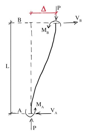
Figure 1. Column segment with length and axial force experiencing relative sway between its ends.
We can think of the axial forces, shears and moments shown above as the primary actions on the structure consistent with the first-order sway deflection, . Again, notice that the axial forces, are no longer co-linear. As a result, an extra second-order moment is developed at the base of the column,
If is a non-negligible value, we must also consider the additional secondary sway deflection caused my . Since the second-order sway deflection further increases the overall sway, leading to yet more secondary sway, we have a feedback loop that could ultimately lead to collapse.
For a tall flexible structure that may undergo significant sway from one storey to the next (storey drift) under lateral base excitation for example, this has catastrophic potential. Only when we are sure that the first-order sway deflection is negligibly small can second-order deflections be ignored.
The effect is a good example of non-linear structural behaviour arising from geometric non-linearity. The typical method of analysis requires iteration to determine the final value that the sway deflection converges on.
This value of sway deflection may be mathematically stable but represent an unsustainable physical configuration for the column. In other words, the second-order deflection may be so high that the column collapses. Ultimately the deciding factor as to whether collapse will occur is the initial sway deflection, , as this sets in motion the feedback loop that delivers the additional second-order deflection.
Since this is a non-linear structural behaviour wherein the inputs to the structural system are not linearly proportional to the outputs (the structure’s behaviour), superposition should not be used in the analysis.
3.0 P-Delta Analysis Example: Fixed-Free Column
Next, we can demonstrate the iterative nature of analysis with a simple example. Consider a simple column with one end fixed and the other free, subject to a vertical load . We will assume that this column experiences a lateral load at that induces an initial first-order deflection .
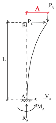
Figure 2. Fixed-free column with axial load and lateral load which induces an initial sway deflection at its free end.
Let’s assume the column has the following parameters,
L = 6000 #(mm) Column height
E = 200*10**3 #(N/mm^2) Young's modulus
I = 2065*10**4 #(mm^4) Iyy for 203UC60 column section
We can determine the Euler buckling load for this column to work out a sensible upper limit for the axial load. We can use the following formula for a fixed-free column,
Note that we’re assuming buckling about the minor axis. This is why we selected from the section tables.
Pcr = pi**2*E*I/(4*L**2) #(N) Critical buckling load
print('The critical buckling load is Pcr = {one} N'.format(one=round(Pcr)))
-> The critical buckling load is Pcr = 283066 N
Let’s assume the column is subject to a compression force of . Let’s also assume that the column is subjected to a lateral force magnitude .
Pv = 0.7*Pcr
Pl = 0.05*Pv
print('The column axial load is Pv = {one} N'.format(one=round(Pv)))
print('The column lateral load is Pl = {one} N'.format(one=round(Pl)))
->The column axial load is ->The column lateral load is
We can calculate the first-order deflection (hereafter referred to as ) due to the lateral load using he standard formula for cantilever deflection,
where is the moment generated at the base of the column by the lateral load .
D1 = (Pl*L**3)/(3*E*I)
print('The first-order deflection, Delta = {one} mm'.format(one=round(D1,1)))
-> The first-order deflection,
We know that this first-order sway deflection induces an additional second-order moment that has a value of at the base of the column. If we examine the internal moment at some distance from the base of the column, we can see that this moment actually varies between at the tip of the column and at the base of the column, with the moment diagram having the same shape as the first-order deflected shape, , Fig. 3.
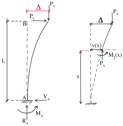
Figure 3. Second-order bending moment.
At this point we can make a simplification and assume that the second-order moment varies linearly between and , Fig.4.
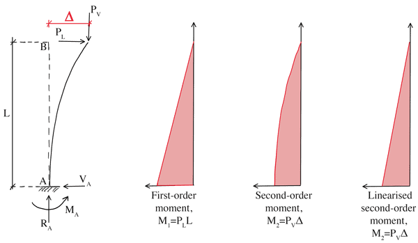
Figure 4. Fixed-free column with first-order, second-order and linearised second-order bending moment diagrams.
If we do this, we can quickly determine the additional deflection induced by the second-order moment using the same equation that was used to calculate ,
where is the first value of second-order deflection calculated. We refer to this value of as the first iteration value, .
M2 = Pv*D1D2 = (M2*L**2)/(3*E*I)
print('The first iteration of second-order deflection, D = {one} mm'.format(one=round(D2,3)))
-> The first iteration of second-order deflection,
Now the iterative nature of the analysis becomes apparent as we need to calculate an additional second-order deflection, induced by this first iteration value, ; in other words, our axial load now generates a further second-order moment, , leading to a second iteration which yields a further second-order deflection, .
The entire process must be repeated yet again with each subsequent value of being added to the preceding value. The iterations continue until the new values of second-order deflection being added become sufficiently small. In this way the second-order deflection converges to its final value. We must then judge the acceptability of the total lateral deflection,
3.1 Writing a function to calculate the secondary deflection
Rather than continuing to perform iterations manually, let’s write a short function to perform the iterations and identify the final second-order deflection.
def P_Delta(Pv,Pl,L,E,I,tol):
  """
  Function to iterate towards the final second-order deflection
  Pv: Vertical load
  Pl: Lateral load
  L: Column length
  E: Young's modulus
  I: Second moment of area
  tol: % change tolerance used to check convergence of deflection

  returns an array of second-order deflection values
  """

  D2Array = np.empty([1,0]) #Initialse an array to hold second-order deflection values
  initMoment = Pl*L #First-order moment
  initDef = (initMoment*L**2)/(3*E*I) #Initial first-order sway deflection
  Dp = initDef #Assign initial sway deflection to variable to be updated in loop

  i=0 #Initialise an iteration counter
  stop = False #Initialise the stop flag
  while stop is False:
    M2 = Pv*Dp #Calculate second-order moment
    D2 = (M2*L**2)/(3*E*I) #Calculate second-order sway deflection
    D2Array = np.append(D2Array, D2) #Save current value of D2
    Dp = D2 #Update the value of sway deflection for next loop iteration

    #Test for convergence
    if i>0:
      diff = np.sum(D2Array) - np.sum(D2Array[0:len(D2Array)-1]) #Change in second-order deflection
      perDiff = 100*diff/(initDef + np.sum(D2Array)) #Change as a percentage of total deflection
      if(perDiff<tol):
        stop = True #Switch stop flag if change within tolerance
    i+=1
  return D2Array
The function defined above continues to perform iterations to identify second-order deflection values until the value of second-order deflection calculated falls below a threshold percentage of the total column deflection. The function then returns the array of all second-order deflections calculated. Next, we need to call the function and print out the array of deflections calculated.
vals = P_Delta(Pv,Pl,L,E,I,0.1) #Call the function to calculate the second-order deflection
print('The second-order deflections obtained on each iteration are:')
print('')
print(vals)
-> The second-order deflections obtained on each iteration are:
[99.4384471 57.24939121 32.96001587 18.97596853 10.92497598 6.28980281 3.62120882 2.08482741 1.20029127 0.69104 0.39785033]
The total deflection is then easily obtained as the sum of the first-order and all second-order deflections.
D2_total = np.sum(vals) #Sum of all second-order deflections across all iterations
print('- The final value of second-order deflection is {one} mm'.format(one=round(D2_total,1)))
print('- {one} iterations were required to reach this value'.format(one=len(vals)))
print('- The total sway deflection is {one} mm + {two} mm = {three} mm'.format(one=round(D1,1), two=round(D2_total,1), three=round(D1+D2_total,1)))
-> The final value of second-order deflection is -> 11 iterations were required to reach this value -> The total sway deflection is
Next we can plot the deflection values on each iteration to observer the convergence.
x = np.arange(1,len(vals)+1) #Define an array of iteration numbers

#Plotting
fig = plt.figure()
axes = fig.add_axes([0.1,0.1,2,1.5])
axes.plot(x,np.cumsum(vals),'-o', label='$\Delta_2$')
axes.plot(x,np.cumsum(vals)+D1,'-o', label='$\Delta*{total}$')
axes.set_xlim([1,len(vals)])
axes.set_ylim([0,1.1*np.cumsum(vals)[-1]+D1])
axes.set_xlabel('Iteration (sec)')
axes.set_ylabel('Deflection (mm)')
axes.set_title('Deflection convergence')
axes.grid()
axes.legend(loc='lower right')
plt.show()
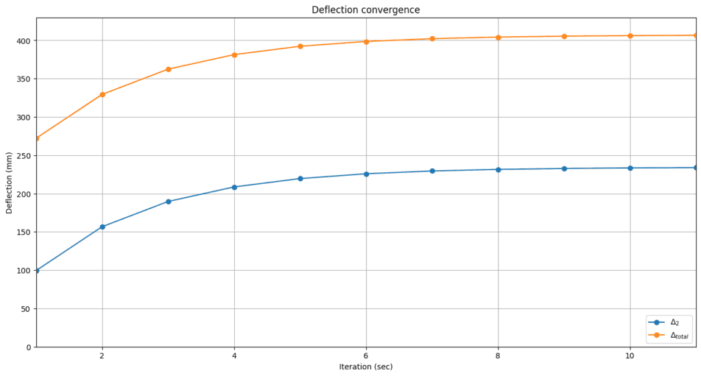
Figure 5. Plot showing convergence of lateral column deflection arising from first and second-order effects.
Now that the additional second-order sway deflection has been determined, subsequent analysis can be carried out to determine the acceptability of the stresses induced. The take away message is the need to be aware of second-order effects when considering the behaviour of slender structures that must resist large axial loads.
4.0 Exploring the P-Delta parameter space
Now that we have a function to calculate the second-order deflection, we can perform a parameter sweep to get a better understanding of the behaviour of the column within the parameter space. After all, we’ve only considered a single combination of axial and lateral load. It would be nice to plot the lateral deflection as a function of these input parameters. We start by defining a range of axial loads as a function of the column critical load and then a range of lateral loads as a proportion of the axial load.
#Axial load as a proportion of the critical load
Axial = np.arange(0.5,1.05,0.05)
#Lateral load as a proportion of the axial load
Lateral = np.arange(0.01,0.11,0.01)
We can now iterate through these values; looping through the axial load with an outer for loop and then the lateral loads with a nested for loop. For every combination of axial and lateral load we will calculate the maximum lateral deflection and the ratio of second to first-order deflection to get a sense of the degree of non-linearity for each parameter combination.
#Define containers to hold calculated values
maxDeflection = np.empty([len(Axial), len(Lateral)])
D2D1*ratio = np.empty([len(Axial), len(Lateral)])

#Initialse a figure (add to it within the loop)
fig, axes = plt.subplots(figsize=(15,15),nrows=2,ncols=1)

#Cycle through each axial load
for i, pv in enumerate(Axial):
  Pv = pv*Pcr #Axial load for this range of iterations

  #Cycle through each lateral load
  for j, pl in enumerate(Lateral):
    Pl = pl*Pv #Lateral load for this iteration

    vals = P_Delta(Pv,Pl,L,E,I,0.1) #Call the function
    D2_total = np.sum(vals) #Total second-order deflection
    D1 = (Pl*L**3)/(3*E*I) #First-order deflection
    maxDeflection[i,j] = D1+D2_total #Total deflection
    D2D1_ratio[i,j] = D2_total/D1 #Deflection ratio

  #Add to plots
  axes[0].plot(Lateral,maxDeflection[i,:]/L,'-o', label='Axial = {one}Pcr'.format(one=round(pv,2)))
  axes[1].plot(Lateral,D2D1_ratio[i,:],'-o', label='Axial = {one}Pcr'.format(one=round(pv,2)))

#Tidy up plots
axes[0].set_title('Total lateral def normalised by column length')
axes[0].set_xlim([Lateral[0],Lateral[-1]])axes[0].set_xlabel('Lateral load as proportion of axial')
axes[0].set_ylabel('$\Delta*{total}/L$')
axes[0].grid()axes[0].legend(loc='upper left')
axes[1].set_title('Ratio of second to first-order deflection')
axes[1].set_xlim([Lateral[0],Lateral[-1]])axes[1].set_xlabel('Lateral load as proportion of axial')
axes[1].set_ylabel('$\Delta_2/\Delta_1$')
axes[1].grid()
axes[1].legend(loc='upper left')
plt.show()
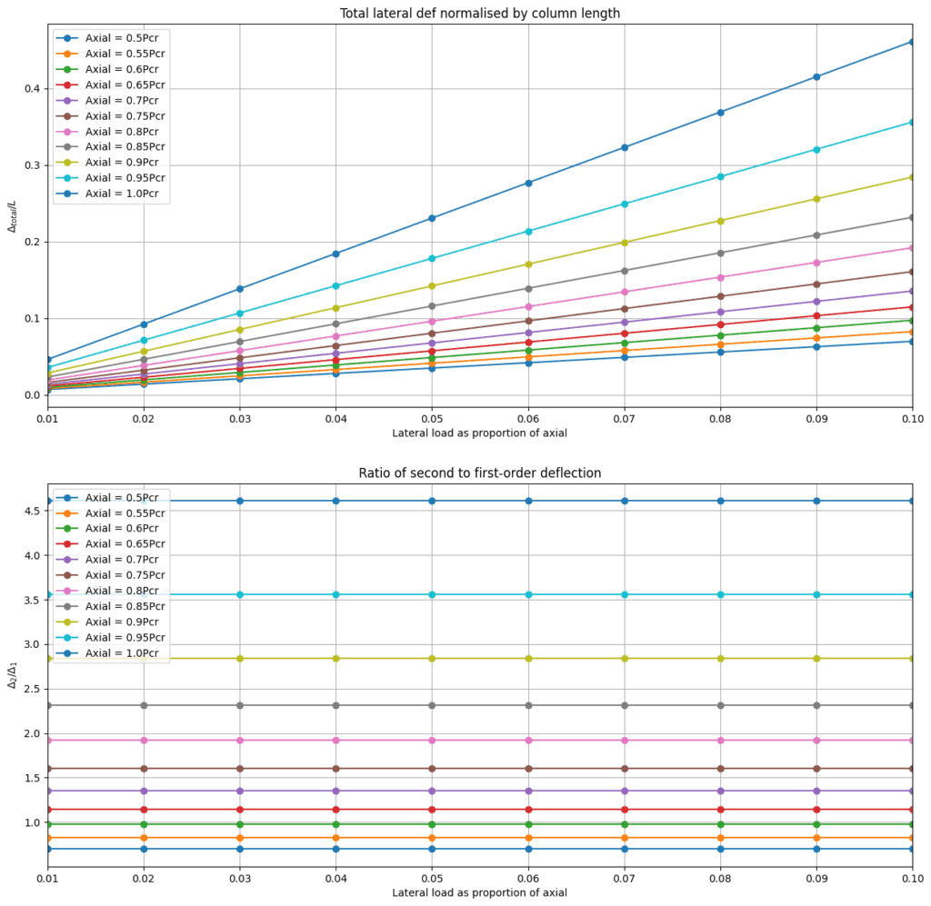
Figure 6. Lateral deflection normalised by column length (top), ratio of secondary to primary deflection (bottom).
We can see from the first plot above that for any particular value of axial load, the total deflection increases linearly with increasing lateral load. This is not at all surprising, however we also note that the rate of increase (slope of each line) increases as the axial load increases.
If we plot the ratio of second to first-order deflection for each load combination (second plot) we can see that for each value of axial load the ratio of second to first-order defection remains constant but as the axial load increases linearly, the increase in the deflection ratios is not linear. We can see this more clearly if we simply plot a single value of deflection ratio against each value of axial load.
fig = plt.figure()
axes = fig.add_axes([0.1,0.1,2,1.5])
axes.plot(Axial,D2D1_ratio[:,0],'-o')
axes.set_xlim([Axial[0],Axial[-1]])
axes.set_xlabel('Axial load as proportion of critical')
axes.set_ylabel('$\Delta_2/\Delta_1$')
axes.set_title('Ratio of second to first-order deflection')
axes.grid()
plt.show()
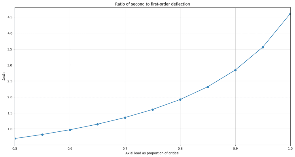
Figure 7. Ratio of secondary to primary deflection for increasing levels of axial load.
We can clearly see that the non-linear deflection exceeds the linear deflection as the axial load increases; the column deflection is quickly dominated by the non-linear component of deflection as the axial load increases. Even though in this example we’ve based our analysis on a column that is particularly prone to non-linear deflection, this highlights the importance of not neglecting second-order sway deflections for slender structures that must resists large axial loads.
5.0 P-Delta analysis for more complex structures
The example above is a pretty contrived but simple and common example used to explain and illustrate effects. However, the question now arises; how do we apply what we’ve learned to more complex structures?
At this point, the road forks and there are two approaches. In each case we assume that you have a model of your structure that you can perform a stiffness method analysis on (check out these courses for building stiffness method analysis tools).
Iterative approach
The first approach is to implement basically the same solution strategy described above:
- Apply any lateral load, to calculate first-order sway deflection, for the structure.
- Manually displace the structural model by applying the nodal displacements to each node in the model according to nodal deflections.
- Apply any vertical loads to the deformed structure to calculate second-order deflections, and note the second-order nodal deflections obtained.
- Displace the structure (from its undisplaced position) according to nodal deflections.
- Apply vertical loads again to the deformed structure to calculate second-order deflections, .
- Repeat steps 4 and 5 until the second-order deflections observed have become negligibly small.
- Calculate the total deflection, .
Geometric stiffness matrix approach
A more sophisticated and efficient approach would be to modify the element stiffness matrix to take into account geometric non-linearity. This will result in an element stiffness matrix that exhibits coupling between the axial force and bending moments in the element. Derivation of this stiffness matrix is beyond the scope of this tutorial, but once obtained, this approach will allow the structure to be solved without iteration. Most commercial frame solvers will have the option of taking into account geometric non-linearity and will calculate the appropriate element stiffness matrix.
Well that’s all for this tutorial. I hope you found it helpful and now have a good understanding of effects as a form of geometric non-linearity and how to calculate them in practice. Remember that you can download the complete Jupyter Notebook for this tutorial for free by clicking the link at the top of this tutorial.
Dr Seán Carroll's latest courses.


Featured Tutorials and Guides
If you found this tutorial helpful, you might enjoy some of these other tutorials.
A Python Programming Roadmap for Structural Engineers
Your complete learning resource guide to getting up and running with Python as a Civil or Structural Engineer.

Dr Seán Carroll
Truss Analysis using the Direct Stiffness Method
A complete introduction to the Direct Stiffness Method for truss analysis with a detailed numerical example

Dr Seán Carroll


