Building a Beam Deflection Calculator in Python

1.0 Beam Deflection Calculator – Project Overview

In this project, we’ll build a beam deflection calculator that can generate beam deflections by directly integrating the bending moment diagram. Since our approach will require a complete bending moment diagram, we’ll add this code onto the end of our Shear Force and Bending Moment Diagram Calculator. So at the end of this project, the final result will be a complete beam analysis code that calculates beam reactions, shear forces, bending moments and deflections.

In our previous beam analysis project, we were limited to analysing statically determinate beams since we relied on the equations of statics. The technique we’ll use for calculating deflection in this project is not limited to statically determinate structures, although you will need a complete bending moment diagram to integrate.

This Python mini-project is accompanied by a complete HD video series. You can access the full playlist for free, by enrolling in the project. In the video series, we’ll walk through the build process line by line. So you can build along with me or if you prefer, just download the finished Python code after you enrol in the project.

I recommend reading through this post (which is a summary of the full project) to get a good overview of the build process and then working through the complete project in more detail.

Building a Beam Deflection Calculator

In this Python project, we build a Beam Deflection Calculator using numerical integration

After completing this project...

You will understand how we can use the bending moment diagram to calculate the deflection of a structure
You will be able to formulate and implement a numerical integration using Python
You will be comfortable building data visualisations using the plotting library Plotly
You will be able to apply what you learn to automate other routine engineering calculations

If you’re new to Python, don’t worry – you don’t need to be a Python programmer to complete this project! Complete beginners can work through this project and pick up the programming basics along the way. If you need help getting your coding environment setup, check out this lecture (part of another course but covers what you need to get up and running). So, with all of that out of the way, let’s get into it.

2.0 Our Approach to Building a Beam Deflection Calculator

We’ve seen in a previous tutorial how we can calculate beam deflections by analytically integrating the differential equation of the deflection curve. We saw first how we could do this by establishing expressions for the internal bending moment as a function of $x$ . Then, we implemented Macauley’s Method to speed up the process by reducing the amount of analytical integration required.

In this project, we’re going to take a different approach. We will still integrate the differential equation of the deflection curve, but we’ll leave the analytical integration to one side and perform our integration numerically. This numerical approach suits our needs quite nicely as we want a method that requires minimal ‘human intervention’. There will be no need to manually determine an equation for the bending moment as a function of $x$ because we already have the bending moment magnitude at each position along the beam. As mentioned above, another strength of this approach is that because all we require as an input is the bending moment diagram, our deflection calculation is not limited to statically determinate structures.

In addition to integrating the differential equation of the deflection curve numerically, we will need to implement some logic along the way that uses our structures’ boundary conditions to ensure we end up with a valid deflected shape, but more on that later.

3.0 Numerical Integration of the Bending Moment Diagram

In this section, we’ll discuss the basic idea of numerical integration and then use this knowledge to build a Python function that integrates the bending moment diagram. Our Python function will return the rotation and displacement at each position along the beam.

3.1 The basic idea – trapezoidal rule

Before we think about numerical integration applied to our specific problem, let’s revisit the basics. We could use several schemes, but one that most people have come across at some point is the trapezoidal scheme or trapezoidal rule. Remember that in the simplest of terms, integration is a way of determining the area under a line. So, let’s imagine some function of $x$ sampled at points $[x_0, x_1, x_2,…x_n]$ , yielding values of the function, $[f(x_0), f(x_1), f(x_2),…f(x_n)]$ , Fig. 1 below.

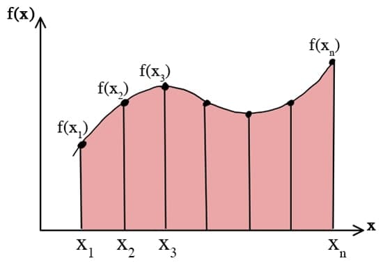
Beam Deflection Calculator_1 | EngineeringSkills.com

Figure 1. Function sampled at equally spaced intervals.

The trapezoidal rule says that the area beneath the line made up by joining the sample values of the function is approximated as,

\text{Area} = \int_{x_0}^{x_n} f(x)\:\mathrm{d}x \approx \frac{\Delta_x}{2}\left[f(x_0) + 2f(x_1) + … +2f(x_{n-1}) + f(x_n) \right] \tag{1}

where $\Delta_x = x_n - x_{n-1}$ , the interval between sampling points (assumed to remain constant). So, the trapezoidal rule boils down to,

\text{Area}\approx \frac{\Delta_x}{2}\left[\text{first sample} + \text{last sample} + 2(\text{sum of all samples in between)} \right] \tag{2}

And if we only have two sample points, i.e. a ‘first’ and ‘last’, we have,

Area \approx \Delta_x\times \frac{f(x_{i-1}) + f(x_{i})}{2} = \text{base length}\times \text{average height} \tag{3}

which we can quite clearly see is the area of a rectangle, Fig 2. This is going to be the basic scheme we use to perform our numerical integration.

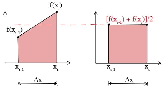
Beam Deflection Calculator_2 | EngineeringSkills.com

Figure 2. The trapezoidal rule applied to a function with two sample points (left), area of rectangle obtained using the trapezoidal rule (right).

Now we can return to our specific challenge; let’s rearrange the differential equation of the deflection curve,

\frac{\mathrm{d}^2v}{\mathrm{d}x^2} = \frac{M}{EI} \tag{4}

Now consider plotting values of $M/EI$ , which is just a scaled version of our bending moment diagram.

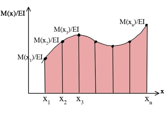
Beam Deflection Calculator_3 | EngineeringSkills.com

Figure 3. Plot of $M(x)/EI$ versus $x$ with $n$ sample points.

Before we can obtain deflections, we must perform an integration to get the rotations,

\theta(x) = \frac{\mathrm{d}v}{\mathrm{d}x} = \int \frac{M}{EI} \mathrm{d}x \tag{5}

We do this by ‘stepping’ through the $M/EI$ diagram and applying the trapezoidal rule to each pair of $M/EI$ values. So, to obtain $\theta_1$ for example,

\theta_1 = \theta_0 + \underbrace{\frac{\Delta_x}{2}\left(\frac{M_0}{EI} + \frac{M_1}{EI} \right)}_{\text{trapezoidal rule}} \tag{6}

After we generalise this equation for any two values of $M/EI$ we obtain,

\boxed{\theta_i = \theta_{i-1} + \frac{\Delta_x}{2}\left(\frac{M_{i-1}}{EI} + \frac{M_i}{EI} \right)} \tag{7}

Notice that to start this whole process off, we needed to provide some value for $\theta_0$ . We essentially have to guess this value! If the value is incorrect, then everything that follows, rotations and deflections will be incorrect too. So we’ll discuss how to address this below. For now, let’s assume we’re happy with the initial value of rotation and proceed to calculate deflections. We need to apply the integration process to our rotation values,

v_1 = v_0 + \frac{\Delta_x}{2}(\theta_0 + \theta_1) \tag{8}

Notice here we also need to provide a starting value for deflection, $v_0$ . If we start our integration at a support, we can safely assume that this value is zero. So generalising our equation we have,

\boxed{v_i = v_{i-1} + \frac{\Delta_x}{2}(\theta_{i-1} + \theta_i)} \tag{9}

After processing all values of $\theta$ , we obtain deflection values for each point along our beam.

3.2 Building a numerical integration function

Now that we understand the basic logic involved in the numerical integration and how to apply it in principle to our problem, we can capture this with some Python code (remember we’re just getting an overview here – refer to the video tutorials above for line by line explanation). For now, we’ll just focus on building a function that takes as its inputs,

the values of bending moment
the flexural rigidity, $EI$
the spacing between sample points, $\Delta x$
the initial rotation and deflection, $\theta_0$ and $v_0$

Our function will process this information and return a rotation and deflection for each sample point along the beam. The reason we’re capturing this logic in a function is so that we can call the function multiple times as we search for the correct initial rotation (discussed below). The complete function is shown in the code block below. Note that some setup code is required before this function, so refer to the video tutorial for the full setup details.

def calcDeflection(M, EI, delX, theta_0, v_0):                
  #Re-assign input arguments to variables used in function    
  theta_im1 = theta_0 #Initial rotation    
  v_im1 = v_0 #Initial displacement     

  #Initialise containers to hold Rotation and Deflection    
  Rotation = np.zeros(len(X))    
  Rotation[supportIndexA] = theta_im1    
  Deflection = np.zeros(len(X))    
  Deflection[supportIndexA] = v_im1     

  #Loop through data and integrate (Trapezoidal rule)    
  for i, m in enumerate(M[supportIndexA::]):        
    ind = i + supportIndexA #Take account of fact that support A might not be at start of beam        
    if i > 0:                    
      M_im1 = M[ind-1]            
      M_i = M[ind]                    
      M_avg = 0.5*(M_i + M_im1)                     

      theta_i = theta_im1 + (M_avg/EI)*delX #Integrate moment values to get rotations                                 
      v_i = v_im1 + 0.5*(theta_i+theta_im1)*delX #Integrate rotation values to get displacements             

      #Store data            
      Rotation[ind] = theta_i                    
      Deflection[ind] = v_i             

      #Update values for next loop iteration            
      theta_im1 = theta_i                 
      v_im1 = v_i                

  return Rotation, Deflection

In lines 4 and 5, we’re simply renaming some of the input arguments; the ‘im1’ in the name stands for $i-1$ . Next, lines 8 to 11 define some data containers to hold our rotation and deflection values. We also assign our initial $\theta_0$ and $v_0$ values at the location in the array that corresponds to the location of the beam support (again, I dig into this more in the video tutorial).

In lines 14 to 30, we iterate through each value from the array of bending moment values (calculated previously) and perform the numerical integration discussed above. Finally, we return the calculated arrays of rotation and deflection values from the function on line 32. Now that we have a function to perform the numerical integration, we need to write the logic that will call this function.

4.0 Identifying the correct initial rotation

So far, we’ve talked about our deflection calculation in an abstract way; let’s base our remaining discussion on a specific beam. Consider the beam below with a cantilever overhang on each side. For now, we’ll ignore the overhang to the left of support A.

Macauley's Method 4 | EngineeringSkills.com

Figure 4. Statically determinate beam with cantilever overhangs to the left and right subject to a range of external actions.

As we said previously, the biggest weakness in our solution so far is that we need to guess a value for the initial rotation, i.e. the rotation at support A. If the wrong value is selected, then all that follows, including our beam deflections, will be incorrect. In this section, we’ll discuss how to address this and determine the correct initial rotation. Our approach will be iterative. We will initially guess a random value for $\theta_0$ and progressively refine our estimate until will arrive at an acceptable value.

4.1 The basic idea – minimising the error

After we guess the initial rotation, we will call our function and calculate the beam deflection. Once we have a deflection, we need to judge its accuracy and, therefore the accuracy of our guess. Fortunately, one thing we know for sure is that the deflection is zero at support B. So this becomes our test; the vertical deflection at the right support becomes our error. All we need to do is keep changing our initial rotation value, calculating the beam deflection and checking if the error is zero or close enough that we’re happy with the approximation.

Next, we need to think about how to alter our guess based on the value of deflection (error) observed at B. If the deflection at B is above the line, we should increase the rotation at A, which will rotate the whole deflected shape such that the deflection at B is reduced back down towards zero. If the deflection at B is below the beam, we should do the reverse and reduce the initial rotation to rotate the deflected shape back up towards zero.

In terms of coding, we’re going to tackle this in two steps. First, we’ll write some code that checks whether increasing or reducing our initial guess reduces the error. Once we know the direction to sweep through rotation values, we’ll call another function that determines the actual value of $\theta_0$ that leads to the smallest error at B.

The code below makes reference to two important parameters that we can tweak to refine our deflection estimates; initRot and deltaRot. initRot is the initial rotation value; the closer it is to the correct value, the fewer iterations are required to calculate the correct initial rotation. deltaRot is the amount by which we change the initial rotation estimate on each iteration of our test. The smaller deltaRot is, the closer we can get to the correct initial rotation value, but the more iterations will be required to get there. You should play around with these values in your final code.

In lines 3-6 below, we’re writing a for loop that will calculate and store the deflection at support B for three different initial rotation values;

our initial guess,
slightly below the initial guess,
slightly above the initial guess.

This allows us to test whether reducing or increasing the initial rotation leads to a smaller or larger deflection error at support B, which we’re testing on lines 8 to 16.

Notice that on lines 11 and 16, we’re calling a function, zeroCrossing() that we haven’t written yet. This function is called with a different value of deltaRot, depending on whether or not we need to continue increasing or reducing our initial rotation. This function returns a single value which we assign to a variable called solvedInitRotation. This is our final estimate of the correct initial rotation at support A.

This allows us to call the deflection calculation function one last time on line 19 and pass in the correct value of the initial rotation. Therefore the deflections and rotations returned on line 19 are the final ‘correct’ values or, in other words, our best approximation.

#Test whether reducing or increasing initial rotation leads to reduction in disp error at other support
testDef = np.zeros(3)
for i, r in enumerate([initRot-deltaRot, initRot, initRot+deltaRot]):    
  Rotation, Deflection = calcDeflection(M, EI, delX, r, initDef)    
  testDef[i] = Deflection[supportIndexB]        

if(abs(testDef[0])<abs(testDef[1])):    
  #Need to test in the negative rotation direction by reducing the initial rotation guess    
  print('Need to test in the negative direction')        
  solvedInitRotation = zeroCrossing(Deflection, -deltaRot, initRot, initDef)             
elif(abs(testDef[2])<abs(testDef[1])):    
  #Need to test in the positive rotation direction by increasing the initial rotation guess     
  print('Need to test in the positive direction')        
  solvedInitRotation = zeroCrossing(Deflection, deltaRot, initRot, initDef)       

#Run the deflection calculation with the solved value of initial rotation
Rotation, Deflection = calcDeflection(M, EI, delX, solvedInitRotation, initDef)    
print('Solved initial rotation is {one}'.format(one=solvedInitRotation))
print('The error in displacement at support is {one}'.format(one=Deflection[supportIndexB]))

4.2 Building a function to find the initial rotation

Now we need to write the function zeroCrossing(), which will take as its inputs the deflection values, the deltaRot value (positive or negative as determined by the code above), and the initial rotation and deflection values at support A. The complete function is shown below.

def zeroCrossing(Deflection, guessStep, initRot, initDef):    
  """    
  Find the value of initial rotation that minimised deflection at right side support by identifying where error crosses zero.    
  """        

  #If the deflection error is positive    
  if Deflection[supportIndexB]>0:        
    errorIsPositive = True #Set flag for error sign                

    #Keep testing lower initial rotation values until error turns NEGATIVE        
    while errorIsPositive:            
      initRot = initRot + guessStep            
      Rotation, Deflection = calcDeflection(M, EI, delX, initRot, initDef)                        

      #If error has turned NEGATIVE, switch the flag to allow loop to stop            
      if Deflection[supportIndexB]<0:                
        errorIsPositive = False                
        solvedInitRotation = initRot #Save the 'solved' value that minimised the error        

  #Else if deflection error is negative    
  elif Deflection[supportIndexB]<0:        
    errorIsPositive = False #Set flag for error sign                

    #Keep testing lower initial rotation values until error turns POSITIVE        
    while not errorIsPositive:            
      initRot = initRot + guessStep            
      Rotation, Deflection = calcDeflection(M, EI, delX, initRot, initDef)                        

      #If error has turned POSITIVE, switch the flag to allow loop to stop            
      if Deflection[supportIndexB]>0:                
        errorIsPositive = True                
        solvedInitRotation = initRot #Save the 'solved' value that minimised the error        

  return solvedInitRotation

This function’s basic approach is to calculate the deflection at support B and test whether it has changed sign since the previous calculation. The while loop will run, successively altering the initial rotation value until the error changes sign. This indicates that between the previous and current loop iterations, the error passed through zero. When this happens, the value of initRot is saved and returned as the ‘solved for’ initial rotation. The smaller the step size, deltaRot, the closer we’re likely to get to the theoretically correct initial rotation. Zero-crossing is a pretty common and simple algorithm we can use to identify when some quantity is zero, or very close to zero.

5.0 Reversing integration direction for deflection of the left side cantilever

At this point, we have produced a reasonable approximation of the beam’s deflection to the right of support A, including the cantilever region to the right of support B. However, we also need our calculator to evaluate cantilever defections to the left of support A. Fortunately, we can use the initial rotation we’ve already calculated for support A and simply integrate in the reverse direction from A out to the left end of the beam.

5.1 Writing the code to identify the left overhang deflection

The code block below shows the reverse integration. This code is almost identical to the code we wrote in our calcDeflection() function above. In particular, note the moment value assignment on lines 13 and 14. Because we are integrating to the left, as we iterate through our moment values, we’re access values with smaller and smaller indices in the array. It’s also worth noting that we only need to access this code if there is a cantilever overhang to the left of the leftmost support. This condition is captured in line 2 by checking if dimension A (specified previously) is not equal to zero.

if A!=0:    
  print("There is an overhand on the left side - solve for deflection by integrating in reverse direction")        

  theta_im1 = -solvedInitRotation #Rotation on other side of support A    
  v_im1 = 0 #Vertical deflection at support A     

  #Generate a range of indices in reverse direction from support A to left endge of beam    
  reverseRange = np.arange(supportIndexA-1,-1,-1)      

  #Loop through data and integrate (Trapezoidal rule) - REVERSE DIRECTION    
  for i in reverseRange:                                
    M_im1 = M[i+1] # Assign previous value of M (reverse direction)        
    M_i = M[i] #Assign current value of M (reverse direction)        
    M_avg = 0.5*(M_i + M_im1)                   

    theta_i = theta_im1 + (M_avg/EI)*delX #Integrate moment values to get rotations                             
    v_i = v_im1 + 0.5*(theta_i+theta_im1)*delX #Integrate rotation values to get displacements                

    #Store data        
    Rotation[i] = theta_i                
    Deflection[i] = v_i         

    #Update values for next loop iteration        
    theta_im1 = theta_i             
    v_im1 = v_i

6.0 Plotting the beam deflection

All that remains is to plot the deflections. We’ve discussed the plotting code in our previous shear and moment diagram project, and I review it in the video tutorial above, so for brevity, I won’t discuss it here. We’ll simply plot the deflection below. To obtain these deflections, I’ve used a value of $200\times 10^{6}\:N/m^2$ for Young’s Modulus and assumed a rectangular beam cross-section $0.2\:m$ wide and $0.5\:m$ deep.

Beam Deflection Calculator_5 | EngineeringSkills.com

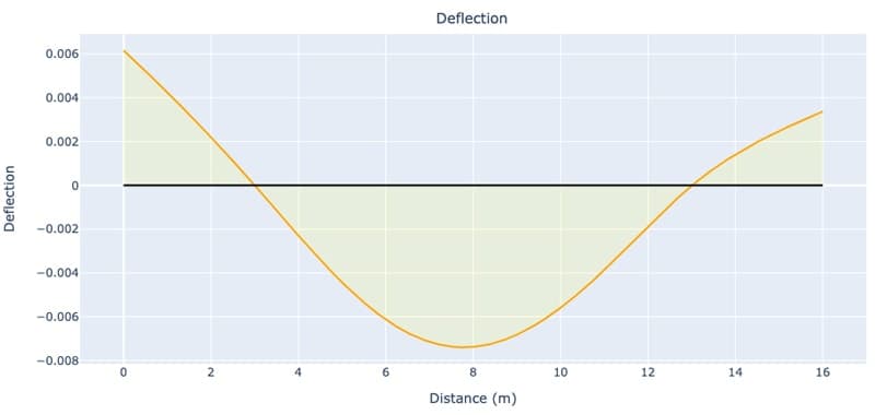
Figure 5. Approximation of the beam deflected shape using the beam deflection calculator.

7.0 Comparing our numerical deflection with an analytical solution

The beam we introduced above was the subject of our Macauley’s Method example in a previous post. This presents us with a convenient validation opportunity. It’s always a good idea to perform some kind of validation exercise whenever you develop any new code. So that’s what we’ll do here by comparing the deflections calculated using Macauley’s Method with those obtained from our numerical deflection estimate. We’ll actually take the opportunity to perform two validation exercises, one on each of the beams analysed in our Macauley’s Method post.

7.1 Example 1 – Simply supported beam without cantilevers

Let’s start with the more straightforward beam analysis.

Simply-supported-beam | EngineeringSkills.com

Figure 6. Simply supported beam subject to a range of loading.

The code block below shows the code that we wrote in the original Macauley’s Method post to plot the deflected shape using the derived deflection equation,

\boxed{EI\: v = \frac{139.375}{6}[x]^3 - \frac{75}{6}[x-3]^3 - \frac{20}{24}[x]^4 - \frac{50}{6}[x-6]^3 + 856.4x} \tag{10}

#Cycle through the structure and calculate the deflection at each point
Deflection_Test = np.zeros(len(X))  #Initialise a container to hold all deflections
for i, x in enumerate(X):        
  deflection = 0     

  #Term 1, 3 and 5    
  if x > 0:        
    #Reaction        
    delta = (139.375/6)*x**3        
    deflection = deflection + delta                

    #UDL        
    delta = -(20/24)*x**4        
    deflection = deflection + delta                

    #C1        
    delta = -856.4*x        
    deflection = deflection + delta            

  #Term 2 - 75kN point load    
  if x-3 > 0:        
    delta = -(75/6)*(x-3)**3        
    deflection = deflection + delta     

  #Term 4 - 50 kN point load    
  if x-6 > 0:        
    delta = -(50/6)*(x-6)**3        
    deflection = deflection + delta     

  #Store shear and moment for this location    
  Deflection_Test[i] = deflection/EI

If we input the beam and loading details for this structure into our beam analysis notebook, we can plot both deflections on the same set of axes, Fig. 7. We can see that the numerical approximation of deflection obtained using our beam deflection calculator is in very close agreement with the analytical solution obtained using Macauley’s Method; so close in fact that when we plot the numerical deflection line (yellow) over the line for the analytical solution (green), it completely obscures it.

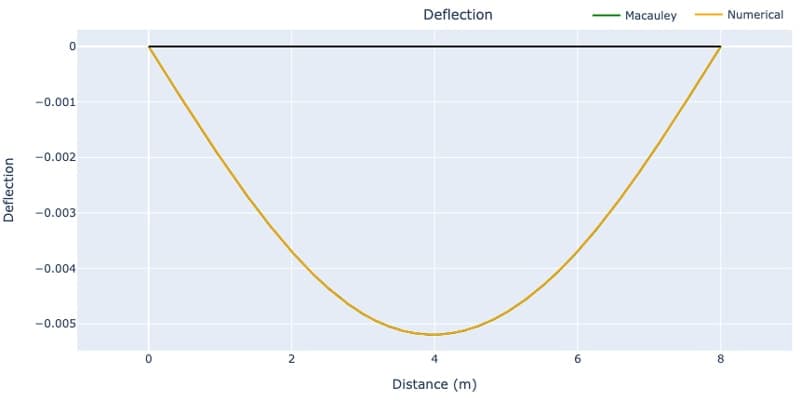
Beam Deflection Calculator_7 | EngineeringSkills.com

Figure 7. Comparison of numerical approximation and analytical solution for beam deflection.

Considering the effort required to implement Macauley’s method, the advantage offered by our new calculator is obvious. With minimal effort, simply inputting the problem parameters, we’ve produced an excellent approximation of the deflection. This gives us great confidence in the code we’ve written.

7.2 Example 2 – Simply supported beam with left and right cantilevers

We’ll compare the numerical and analytical deflections for the beam we started with above (Fig. 4) to conclude our discussion. Again, we’ve derived the Macauley’s Method deflection equation previously,

\begin{align*} v =& \frac{1}{EI}\left \{ -\frac{60}{2}[x]^2 +\frac{123.5}{6}[x-3]^3 - \frac{50}{24}[x-5]^4 - \frac{100}{6}[x-11]^3 \right\} + \\\\ + & \frac{1}{EI} \left \{ \frac{50}{24}[x-9]^4 + \frac{251.5}{6}[x-13]^3 - 765[x] + 2565 \right\} \end{align*} \tag{11}

For completeness, the code used to generate the deflected shape using this equation is shown below.

#Cycle through the structure and calculate the deflection at each point
Deflection*Test = np.zeros(len(X))  #Initialise a container to hold all deflections
for i, x in enumerate(X):        
  deflection = 0     

  #Term 1 and 7    
  if x > 0:        
    #Moment        
    delta = -(60/2)*x**2        
    deflection = deflection + delta                

    #C1        
    delta = -765*x        
    deflection = deflection + delta            

  #Term 2 - Reaction at A    
  if x-3 > 0:        
    delta = (123.5/6)*(x-3)**3        
    deflection = deflection + delta     

  #Term 3 - 50 kN/m UDL acting downwards    
  if x-5 > 0:        
    delta = -(50/24)_(x-5)**4        
    deflection = deflection + delta        

  #Term 4 - 100kN point load    
  if x-11 > 0:            
    delta = -(100/6)*(x-11)**3        
    deflection = deflection + delta            

  #Term 5 - 50 kN/m UDL acting upwards    
  if x-9 > 0:        
    delta = (50/24)_(x-9)**4        
    deflection = deflection + delta            

  #Term 6 - Reaction at B    
  if x-13 > 0:        
    delta = (251.5/6)*(x-13)**3        
    deflection = deflection + delta            

  #Term 7 - C2    
  deflection = deflection + 2565                    

  #Store deflection for this location    
  Deflection_Test[i] = deflection/EI

Comparing the numerical and analytically obtained deflections, Fig. 8, we can again see close agreement, strengthening our confidence in the validity of our calculator output.

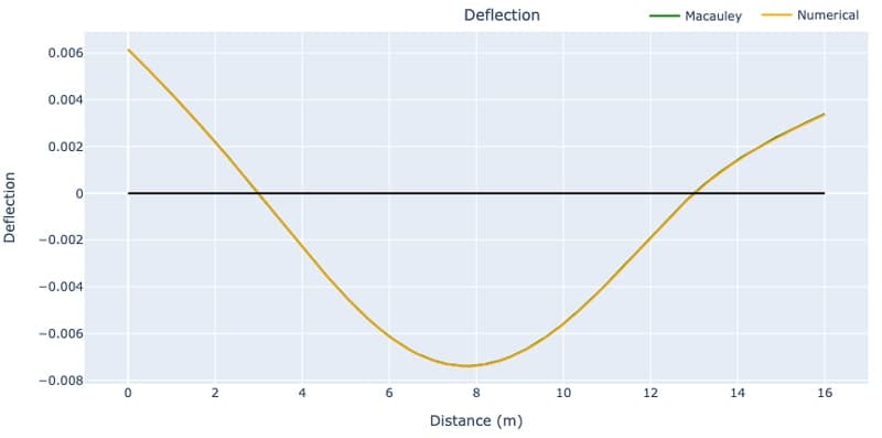
Beam Deflection Calculator_8 | EngineeringSkills.com

Figure 8. Comparison of numerical approximation and analytical solution for beam deflection.

At this stage, you should have a good sense of how we’ve pieced this beam deflection calculator together. Armed with the roadmap in this post, go ahead and work your way through the tutorial videos at the top of the post. These will cover all of the details that we didn’t have space to go into here.

I hope this post has given you a taste for combining basic coding with structural analysis. Programming is a huge force multiplier for your structural analysis knowledge. If you want to dive further into code-based structural analysis, consider the stiffness method course bundle. In these courses, I walk you through building a range of Python analysis tools for analysing 2D and 3D truss systems as well as 2D beam and frame structures. What we discussed in this post is only the tip of the iceberg compared to what you can build!

That’s all for now, see you in the next one!