Building a Shear Force and Bending Moment Diagram Calculator in Python

1. Introducing our Shear Force and Bending Moment Diagram Calculator

Welcome to another Python mini-project. In this project we’re going to build a Shear Force and Bending Moment Diagram calculator using Python in the Jupyter Notebook development environment. Generating the shear force and bending moment diagram for a simple beam with anything other than basic loading can be a tedious and time-consuming process. Once you finish this project, you’ll have a calculator that can produce shear force and bending moment diagrams at the push of a button.

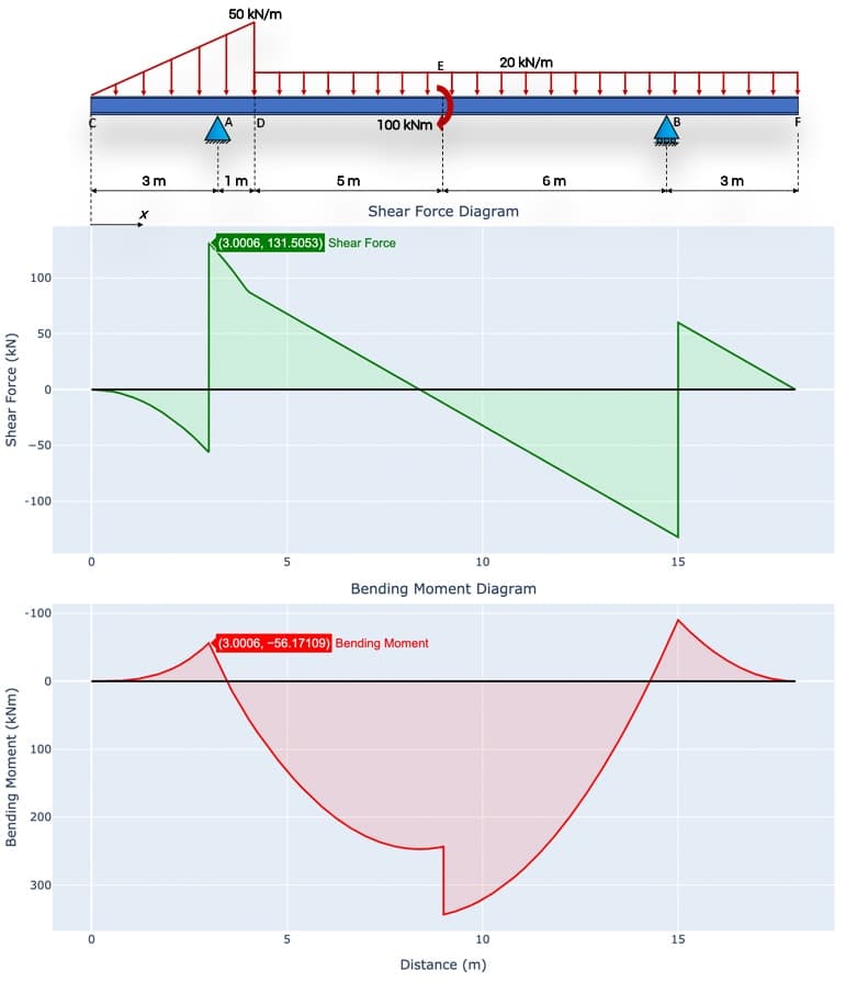
Fig. 1: Shear force and bending moment diagrams generated for the simply supported beam and loading shown (top).

Whether you’re an engineering student or a working engineer, this shear and moment calculator is going to make life a little bit easier for you. For engineering students in particular who are learning how to build shear force and bending moment diagrams, your calculator gives you unlimited examples to test yourself against. The frequent request for ‘example questions’ from students was actually the main motivation to build this calculator in the first place. 

This Python mini-project is accompanied by a complete HD video series. You can access the full playlist for free, by enrolling in the project. In the video series, we’ll walk through the build process line by line. So you can build along with me or if you prefer, just download the finished Python code after you enrol in the project.

As I always say at the start of a new EngineeringSkills project or course – you don’t need to be a Python programmer to complete this project! Complete beginners can work through this project and pick up the programming basics along the way. If you need help getting your coding environment setup, check out this lecture (part of another course but covers what you need to get up and running).

2. The Principle of Superposition and our approach to the build

We’re going to make use of the Principle of Superposition to build our calculator. In the context of our simply supported beam, this simply means that we can determine the influence of multiple loads acting simultaneously by adding together the influences of the same loads acting individually. We used the Principle of Superposition when we were calculating beam deflections from first principles here.

It’s important to note that we can only use the Principle of Superposition when our structural behaviour can be assumed to be linear. If any of the loads on our structure induce non-linear plastic behaviour, application of the superposition principle is no-longer valid. Provided we’re satisfied that the behaviour remains linear, we can use this principle to layer the resulting influences of as many actions as we like.

So for example, we’ll write a function that calculates the reactions from a single point load $P$ located at $x_p$ meters from the left side of our beam. Then we’ll construct a ‘for loop’ that cycles through each of the point loads we’ve specified and calls our function to determine the reactions from each point load acting individually. If we record the reactions from each point load, we can use the Principle of Superposition to add them all together and find the reactions assuming that all of the point loads were acting simultaneously.

We’ll take the same approach when it comes to calculating the shear force and bending moment at each point along our beam. We’ll start by constructing a vector of x-coordinates along our beam. We’ll then write a function to calculate the shear force and bending moment at some distance $x$ along our beam. By calling this function within a loop for each x-coordinate, we’ll build up a range of shear and moment values along the length of our beam. Again, we’ll use superposition to layer together the influence of multiple external forces/moments acting simultaneously.

We’ll build in the ability for our code to calculate the reactions and internal shear forces and bending moments across our structure in response to:

• Point loads,
• Point moments,
• Uniformly distributed loads,
• Distributed loads of linearly varying magnitude (triangular loads)

This should represent the most common forms of beam loading. But after completing the project, you’ll be more than capable of expanding your calculator to other forms of loading.

3. Calculating reactions due to point loads

We’ll walk through the calculation and coding process for point loads in detail here. But once you’ve understood what’s going on for point loads, the process to implement applied moments and distributed loads only required  incremental additions (which we’ll walk through in detail in the video series).

We’ll base our code development on the example structure shown in Fig. 2 below. We analysed this structure in detail here – so refer back to that post for a refresher on the fundamentals of shear force and bending moment diagrams.

Fig. 2: Example structure

Let’s start by importing some standard packages and initialising some data containers to hold our reactions, shear forces and bending moments. We’ll store the cumulative sum of all reactions (from all applied loads) in the ‘reactions‘ array. For now, we’ll store the shear forces and bending moments induced by each applied load in a separate row within a 2D array. We’ll sum up all values at each location (superposition!) just before we plot the shear force and bending moment diagrams. Notice that in lines 8 and 9 below, we are defining the length of each row as len(x). This just means we want a ‘slot’ or space to store a value for each value contained in X, where X is the array of x-coordinates defined elsewhere in our code.

# DEPENDENCIES
import math #Math functionality
import numpy as np #Numpy for working with arrays 

#INITIALISE DATA CONTAINERS
reactions = np.array([0.0,0,0]) #Reactions (Va, Ha, Vb) - Defined as array of floats to hold reactions
shearForce = np.empty([0,len(X)]) #Shear forces at each data point
bendingMoment = np.empty([0,len(X)]) #Bending moment at each data point

Next we’ll specify some analysis parameters. Our code will need to be capable of accommodating beams that have a cantilever overhang on the left and/or the right side. Therefore in addition to specifying a span we also define a distance to the left and right support, $A$ and $B$ respectively. Note that all distances are measured from the left side of the beam.

Point loads will be defined in a 2-dimensional numpy array with each row representing an individual point load. For each point load (row in the 2D array) we specify the location of the force, the magnitude of the horizontal component and the magnitude of the vertical component. In the code below we are specifying a single vertical point load of magnitude $90 \:kN$, acting $6\:m$ from the left side of the beam. The negative sign indicates the load is acting vertically downwards (negative y-direction).

#ANALYSIS PARAMETERS
span = 17 #Span of beam
A = 3  #Distance to left support
B = 13 #Distance to right support point
Loads = np.array([[6,0,-90]])

Next we need to work out the equations required to calculate the reactions. Once we’ve worked this out ‘by hand’, we can capture this logic in code and write a function to perform the task. As our beam is statically determinate, we can use equilibrium equations to determine the three unknown reactions.

Fig. 3: Example structure subject to the point load alone.

Taking the sum of the moments about point A the left hand pin support yields $V_B$,

Now, rather than working in terms of numbers directly, if we instead define

• the distance between $A$ and $B$ as the lever arm of $V_B$ about $A$, $la\_vb$
• the distance to the applied vertical load as $x_p$ and the load itself as $f_y$
• the lever arm of the vertical load about point $A$ as $A-x_p$

we can construct an expression for the reaction $V_B$ that will yield the correct answer for any combination of the values of $x_p$, $A$, $la\_vb$ and $f_y$. This is the expression we’ll bake into our Python code,

Notice that a negative (downward pointing) vertical load to the right of $A$ will generate a positive moment by virtue of the negatively defined lever arm, $A-x_p$. In a similar fashion we can determine suitable expressions for $V_A$ and $H_A$,

We can now capture these calculations in a simply Python function. We will use the function argument ‘n‘ to indicate to the function which point load it should operate on.

def reactions_PL(n):
  xp = pointLoads[n,0] #Location of point load
  fx = pointLoads[n,1] #Point load horizontal component magnitude
  fy = pointLoads[n,2] #Point load vertical component magnitude   

  la_p = A-xp #Lever arm of point load about point A
  mp = fy*la_p #Moment generated by point load about A - closkwise moments are positive
  la_vb = B-A #Lever arm of vertical reaction at B about point A 

  Vb = mp/la_vb #Vertical reaction at B
  Va = -fy-Vb #Vertical reaction at A  
  Ha = -fx#Horizontal reaction at A  

  return Va, Vb, Ha

Now that we have our reactions_PL(n) function written, all we need to do is call it…for every point load on our structure. In our example we obviously only have a single point load, but this may not always be the case. We start on line 2 below by initialising an empty numpy array. We want to store the reactions associated with each point load as we’ll need these later when it comes to calculating the shears and moments resulting from each point load.

Next we set up a for loop to cycle through each point load in our store of pointLoads defined earlier. We’ve also set up an iterator to start at zero and count up by one every time we pass through our loop. Once inside the loop, we call our function for the relevant point load on line 5 and assign the reactions returned to new variables, $va$, $vb$ and $ha$. On line 6 we record these for use later and on lines 9-11, we update our ‘running total’ for the reactions.

PL_record = np.empty([0,3])

for n, p in enumerate(pointLoads):
  va, vb, ha = reactions_PL(n) #Calculate reactions
  PL_record = np.append(PL_record, [np.array([va, ha, vb])], axis=0) #Store reactions for each point load     

  #Add reactions to record (superposition)    
  reactions[0] = reactions[0] + va
  reactions[1] = reactions[1] + ha
  reactions[2] = reactions[2] + vb

When it comes to calculating reactions for any type of loading, we’ll follow this basic architecture; define a function to capture the specifics of the calculation, then call that function in a loop that cycles through each one of the loads/moments we’re concerned with.

4. Calculating shear forces and bending moments due to point loads

Now it’s time to consider shear forces and bending moments at each point along our beam. We’ll focus here on point loads – but the same process is implemented for all loading types. We start by defining a function to calculate the shear and moment at every location for a single point load and then call this function in a loop as we consider each point load individually.

To build a suitable function, let’s start by considering our beam again, Fig. 4 below. There are three possible forces that will influence the internal shear force and bending moment at a point, the reactions at A and B and the point load, $f_y$. If we cut the structure to reveal the internal shear and moment and then evaluate these quantities by considering equilibrium of the sub-structure to the left of the cut, only those forces to the left of the cut will contribute to the shear and moment equations.

Therefore if we cycle along each point (x-coordinate) on the beam, we can check which forces are to the left of the current point (cut location) and add the influence of any forces to the left of the current point to the internal shear force and bending moment. For example consider the three vertical cut locations identified in Fig. 4. below.

Fig. 4: Cut locations that identify three distinct regions of the structure for shear and moment calculation.

Consider cut 1-1, to the right of $V_A$ but to the left of $f_y$. 

By considering equilibrium of this substructure we determine the following expressions for the shear force and bending moment,

We can construct the same equilibrium equations to capture the shear and moment influence of the point load in the event that our cut is to the right of the point load, Fig. 6 below,

Finally, the shear and moment are calculated for sections to the right of $V_B$ as,

Now we can capture these equations in a shear and moment calculating function, shear_moment_PL(n). It will again take n as a parameter to identify the load on which it must act. When comparing the equations above with those shown in the function below, note that within our Python code, $f_y$ is already defined as a negative number, so some of the signs will differ when they make it into the Python code. Also, when it comes to plotting the bending moment diagram, we have manually reversed the y-axis on our plot such that negative values  (below the line) appear as positive numbers consistent with the typical convention for drawing sagging bending moments as positive.

Taking a closer look at the function defined below we see that on lines 3-6 we are simply redefining some variables associated with the current point load with short names making our code easier to read. On lines 9 and 10, we are initialising arrays of zeros, essentially starting by setting the shear and moment at every location to zero, so that we can override with calculated values later.

We setup our for loop on line 11 to cycle along each x-coordinate on the beam. Now inside the loop, on lines 12 and 13, we initialise the specific value of shear and moment for this location to zero. Then from lines 15 to 28 we progressively add to the shear and moment at this location by checking which of the three forces have an influence. As discussed above, we determine this simply by checking which of the three forces is to the left of the current value of $x$ (recall that $A$ and $B$ are the distances to the left and right supports respectively while $x_p$ is the distance to the point load location).

Once we’ve calculated a suitable value of shear and moment for the current $x$ location by superimposing the influences of $V_A$, $V_B$ and $x_p$, we store those values on lines 31 and 32. Finally after looping through all x-coordinates and storing the values of shear and moment at each location, we return the complete record of shear forces and bending moments out of the bottom of the function.

def shear_moment_PL(n):
  xp = pointLoads[n,0] #Location of point load    
  fy = pointLoads[n,2] #Point load vertical component magnitude     
  Va = PL_record[n,0] #Vertical reaction at A for this point load    
  Vb = PL_record[n,2] #Vertical reaction at B for this point load

  #Cycle through the structure and calculate the shear force and bending moment at each point    
  Shear = np.zeros(len(X)) #Initialise a container to hold all shear force data for this point load    
  Moment = np.zeros(len(X)) #Initialise a container to hold all moment force data for this point load    
  for i, x in enumerate(X):
    shear = 0 #Initialise the shear force for this data point
    moment = 0 #Initialise the bending moment for this data point 

    if x > A:
      #Calculate shear and moment from reaction at A    
      shear = shear + Va
      moment = moment - Va*(x-A)

    if x > B:
      #Calculate shear and moment from reaction at B    
      shear = shear + Vb
      moment = moment - Vb*(x-B)

    if x > xp:
      #Calculate shear and moment from point load    
      shear = shear + fy
      moment = moment - fy*(x-xp)

    #Store shear and moment for this location
    Shear[i] = shear
    Moment[i] = moment

  return Shear, Moment

The next task is to call our shear force and bending moment calculator function from within another loop for each externally applied point load on our structure. We handle this in exactly the same way as we handled calling our reaction_PL function. In the code block below, we set up our for loop on line 3, call the shear and moment calculator function on line 4 and assign the output from the function to variables Shear and Moment. Note that Shear and Moment are each an array of numbers and not single values. The last step on lines 5 and 6 is to store the Shear and Momentvalues as new rows in our larger data structures shearForce and bendingMoment which we’re using to record the shears and moments for every individual action applied to the structure.

At this point the basic process is complete and we’ve implemented the logic for our shear force and bending moment calculator to handle multiple point loads applied along our structure. The good news is that from here on, we basically just rinse and repeat this workflow and implement the exact same architecture for all other forms of loading.

#Calculate the shear force and bending moment at each datapoint due to point load
for n, p in enumerate(pointLoads):
  Shear, Moment = shear_moment_PL(n)
  shearForce = np.append(shearForce, [Shear], axis=0) #Store shear force record for each point load
  bendingMoment = np.append(bendingMoment, [Moment], axis=0) #Store bending moment record for each point load

5. Handling applied moments and distributed loads in our shear force and bending moment calculator

Now that we’ve seen how to build the code to calculate reactions, shear forces and bending moments for point loads, we won’t dive into the corresponding code for point moments and distributed loads in this post. This is fully covered in the video series above. Instead, in this section we’ll briefly demonstrate how the outputs from each load type analysis combine to produce the final shear force and bending moment diagram.

Fig. 8 below shows the Principle of Superposition in action. In plots A-C we can see the shear force diagrams produced by applying each action individually while in plot D we can see the shear force diagram produced when all actions are applied simultaneously. We can see that the shear force diagram D is simply the summation or superposition of diagrams A-C. Our shear force and bending moment diagram calculator simply repeats the analysis described above for every load type and adds all of the shear force and bending moment diagrams together.

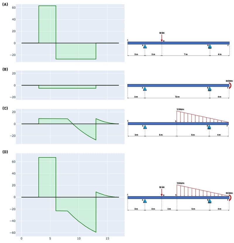
Fig. 8: Superposition of shear force diagrams for point load (A), point moment (B) and linearly varying distributed load (C) to produce the final shear force diagram for all loads acting simultaneously (D).

For completeness I’ve provided the same superposition breakdown in Fig. 9 below for the bending moment diagrams. This type of ‘deconstruction’ of the shear force and bending moment diagrams is particularly helpful for any student trying to refine their understanding of shear and moment diagrams or trying to enhance their understanding of qualitative structural behaviour. 

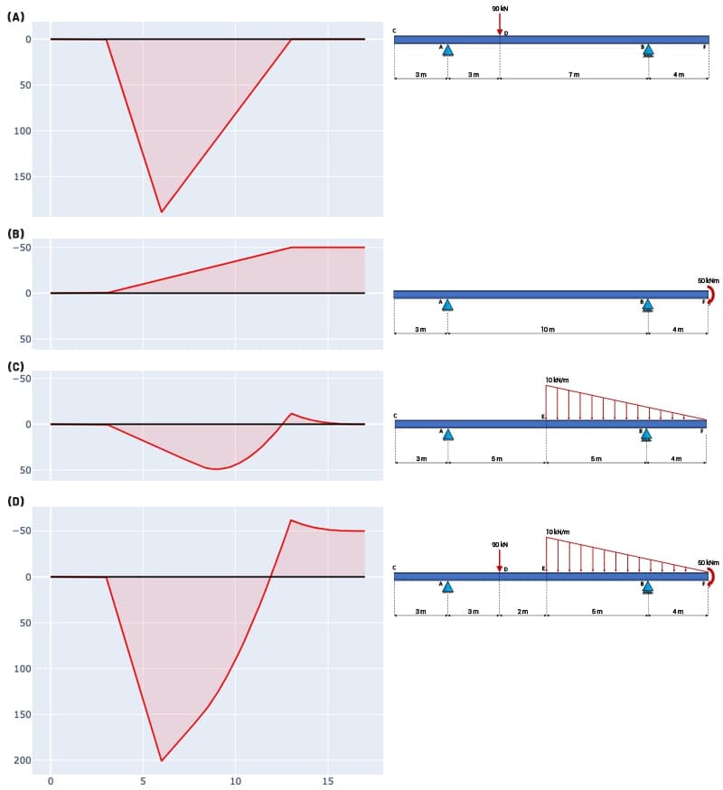
Fig. 9: Superposition of bending moment diagrams for point load (A), point moment (B) and linearly varying distributed load (C) to produce the final bending moment diagram for all loads acting simultaneously (D).

6. The limitations of our shear and moment calculator

Before rapping up this project we should remind ourselves of the limitations of our calculator and suggest possible next steps for advancing the project. The first limitation has already been mentioned above – we’re assuming linear behaviour. This does technically limit the applicability of our calculator but frankly, most initial structural analyses will assume linearity. So it’s not a huge practical barrier. More sophisticated structural analyses that consider geometric or material non-linearity can be performed on later analysis iterations.

By far the biggest limitation of this calculator is the fact that it can only be applied to statically determinate beams. Throughout the build process, we relied solely on the three equations of equilibrium to determine unknown reactions, shear forces and bending moments. At no point did we deploy any more sophisticated analysis techniques. As such, our calculator will ‘break‘ if we try and feed it anything other than a statically determinate simply supported beam. Our shear and moment calculator is a handy tool and a great study aid but it’s not an all singing all dancing structural solver!

To unlock statically indeterminate structures we need to deploy a more sophisticated analysis method – the most commonly used method for computerised structural analysis is the direct stiffness method or more generally the finite element method. You can read an in-depth tutorial on the direct stiffness method here. If you want to build your own structural analysis solver using the direct stiffness method, that’s not limited to statically determinate beams, check out my course, Beam & Frame Analysis using the Direct Stiffness Method in Python (details below).

In terms of next steps, you have a number of options. Obviously you could take the course above and go straight for the Rolls Royce solution! Alternatively, why not take what you know after finishing this project and extend your shear and moment calculator to take into account rotational hinges within the beam. This would be a really good way of adding great functionality and at the same time testing yourself to independently develop some code! Remember, if you can work out how to do something on paper – the hard part is done! Writing some Python code to capture the logic is generally the easy part.

You could consider writing a calculator for 2D frame structures – but in all honesty that sounds like a lot of work! This would not be the best approach – you’d be far better using a stiffness method analysis for this. However, this simple calculator model would map quite nicely onto torsional analysis of a shaft. You could calculate internal torques, angles of twist and shear stresses simply by adapting the approach we’ve taken here. As I write this, that’s sounding like a pretty good project – I might actually do that one.

Well, that’s it for this project. I hope you’ve found this overview tutorial interesting and helpful. If you want to continue working on this project and haven’t done so yet, start watching the video series and building your own version of the shear force and bending moment calculator. As some final food for thought, what other routine calculations can you automate – a typical day of analysis and design is full of calculations we repeat over and over again. Why not invest a little time in building a Jupyter Notebook calculator to free up some time down the line – your future self will thank you!